d <- tibble(
  A = c("X", "Y", "X", "Z", "Z", "X"),
  B = c(1.5, 5.0, 4.5, 2.0, 1.0, 2.0),
  C = c("U", "V", "V", "W", "V", "W")
)4 Untersuchung einzelner Merkmale in R
Übersicht Dataframes für diese Folien
| Name | Inhalt |
|---|---|
d_wb_all |
Weltbank - Alle Länder, alle Jahre |
d_wb_2012 |
Wie d_wb_all, aber nur für das Jahr 2012 |
d_wb_countries |
Wie d_wb_all, aber nur ausgewählte Länder |
d_wb_countries_2012 |
Wie d_wb_countries, aber nur für das Jahr 2012 |
d_ns_bochum_tag |
Tageswerte für Niederschläge in Bochum |
d_ns_bochum_monat |
Monatswerte für Niederschläge in Bochum |
Quellen: https://data.worldbank.org und https://www.dwd.de
4.1 Werte plotten mit geom_col()
Beispieldatensatz
- Mit
tibbleauf die Schnelle einen Dataframe erzeugen - Werte für ein Merkmal mit
c(...)kombinieren - Zeichenketten in Anführungszeichen eingeben
- Mit
<-wird der Dataframe der Variablendzugewiesen
Minimalbeispiel
ggplot(data = d) +
  geom_col(mapping = aes(x = A, y = B))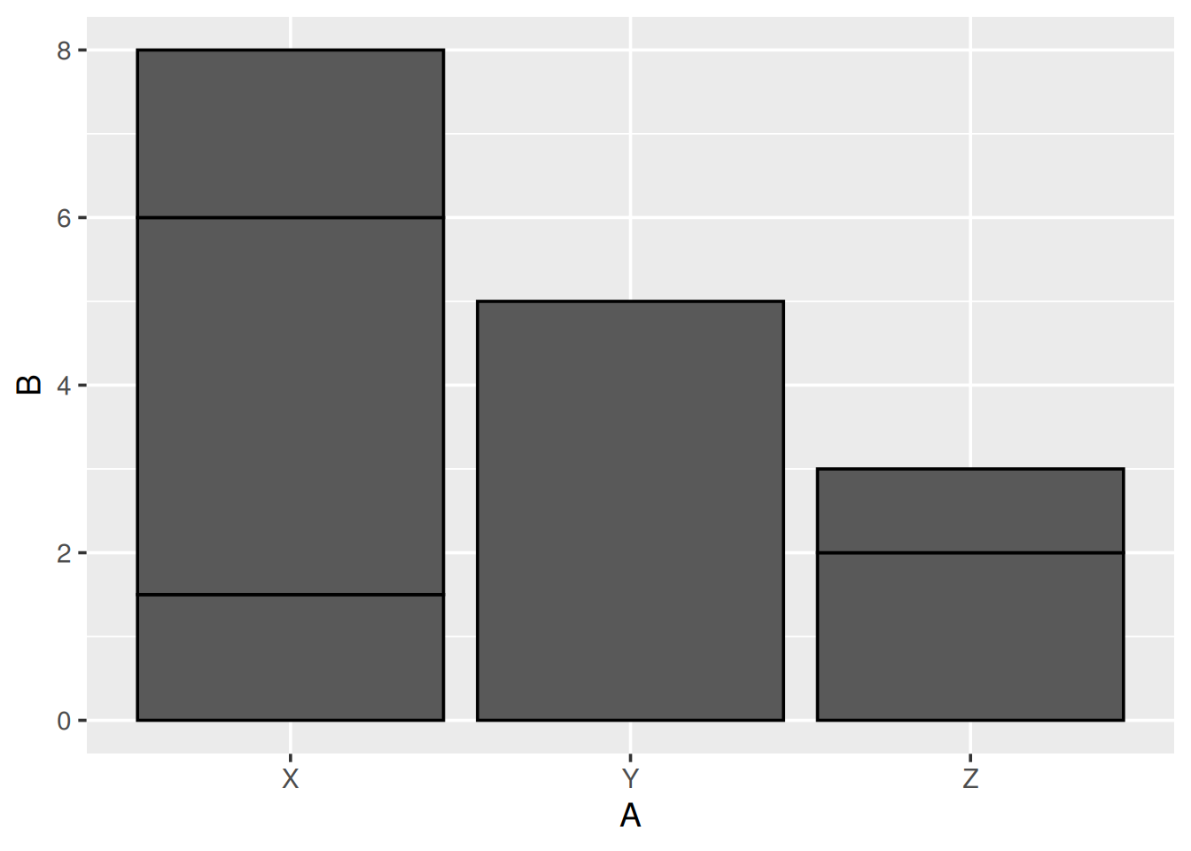
- Höhe der Säule aus Summe der Werte von Merkmal B
Füllfarbe nach drittem Merkmal
ggplot(data = d) +
  geom_col(mapping = aes(x = A, y = B, fill = C))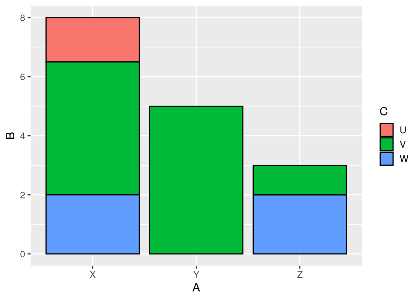
- Mit
fill = <M>Merkmal für Füllfarbe angeben
Nebeneinander
ggplot(data = d) +
  geom_col(mapping = aes(x = A, y = B, fill = C), position = "dodge")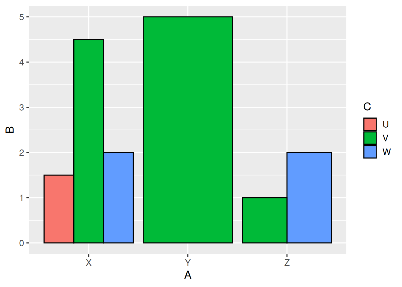
- Nebeneinander anordnen mit
position = "dodge"
Als Balkendiagramm
ggplot(data = d) +
  geom_col(mapping = aes(x = A, y = B, fill = C)) +
  coord_flip()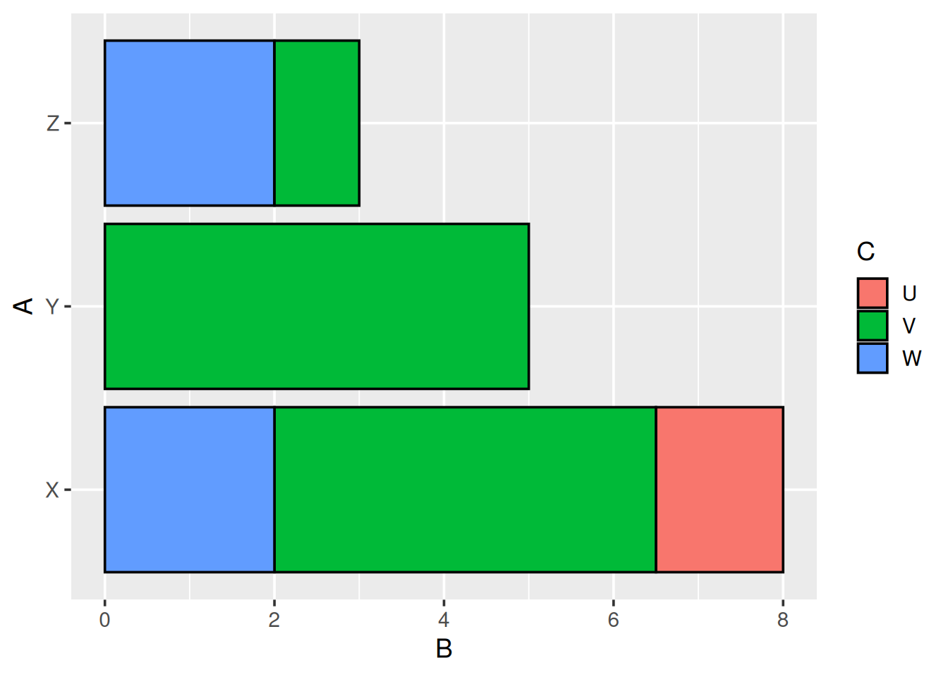
- Mit
coord_flip()Koordinatenachsen vertauschen
Mit echten Daten…
Treibhausgasemissionen (2012)
ggplot(data = d_wb_countries_2012) +
  geom_col(mapping = aes(x = country, y = gge))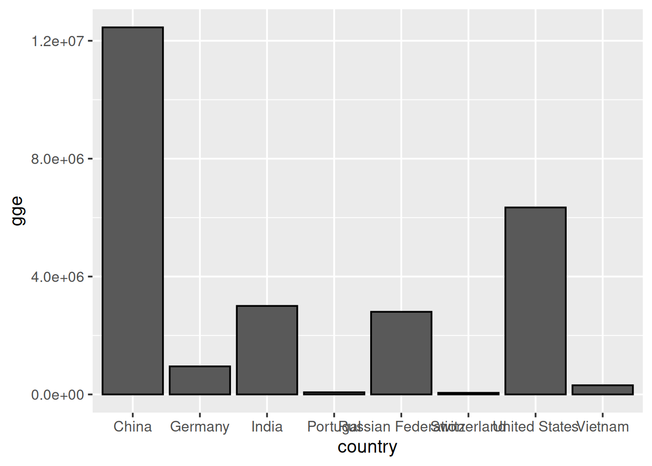
- Zur Erinnerung:
ggesteht für Greenhouse Gas Emissions
Treibhausgasemissionen bunt (2012)
ggplot(data = d_wb_countries_2012) +
  geom_col(mapping = aes(x = country, y = gge, fill = region))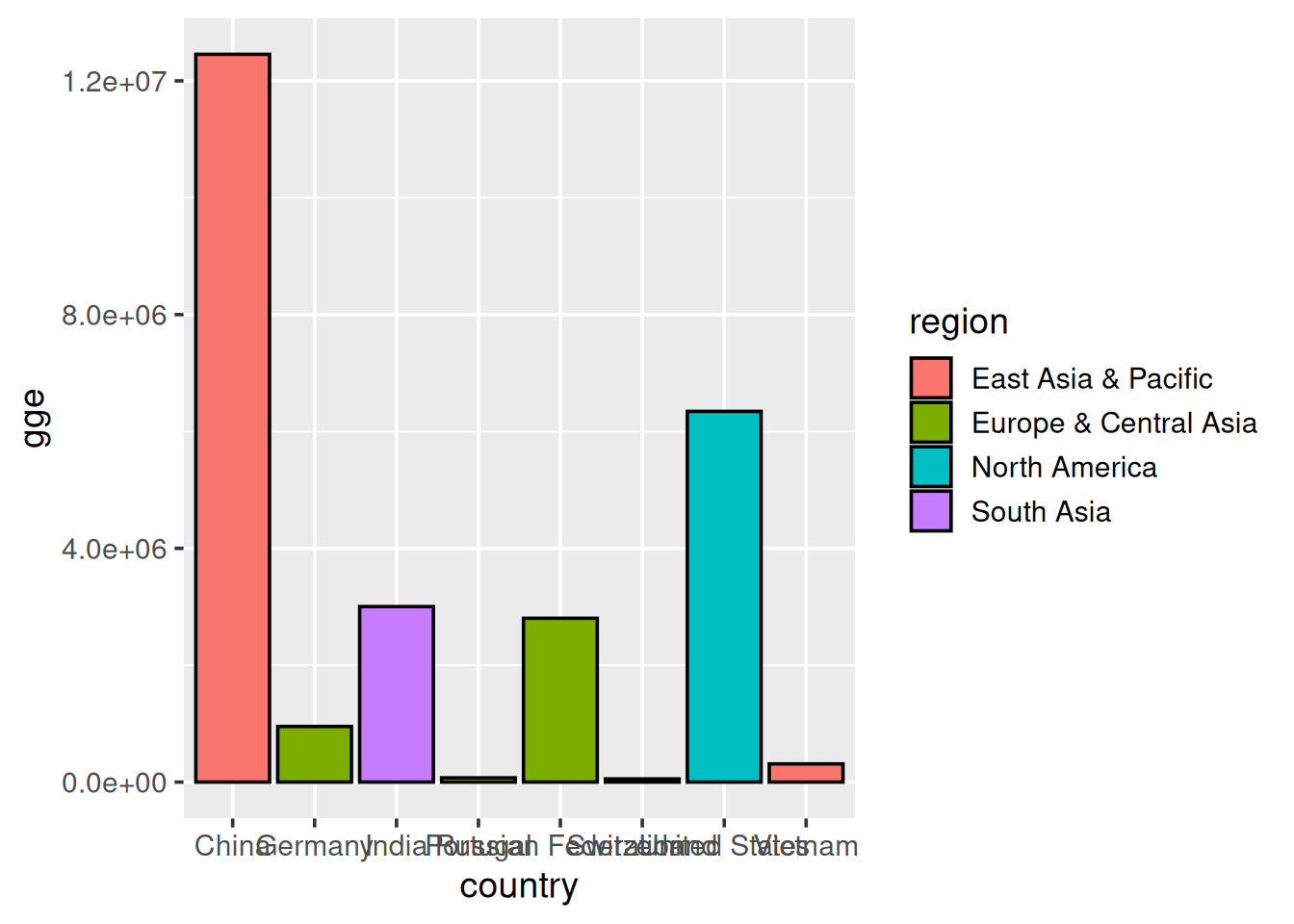
- Nach Weltregion eingefärbt
Treibhausgasemissionen pro Kopf (2012)
ggplot(data = d_wb_countries_2012) +
  geom_col(mapping = aes(x = country, y = gge / pop, fill = region))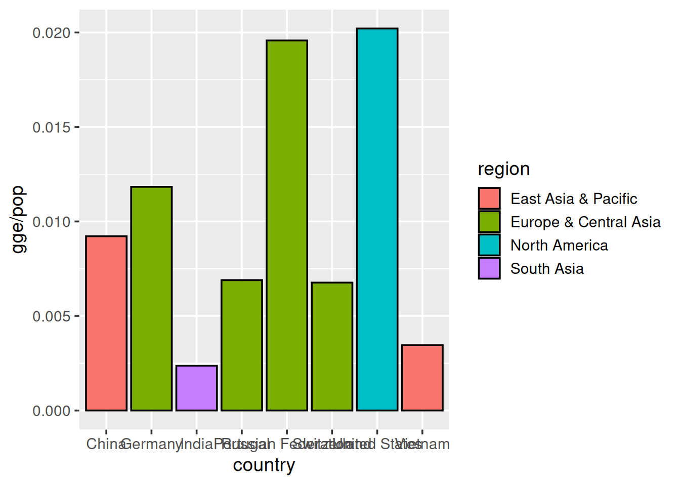
- Rechnen mit Merkmalen:
y = gge / pop
Treibhausgasemissionen über die Zeit
ggplot(data = d_wb_countries) +
  geom_col(mapping = aes(x = year, y = gge, fill = country))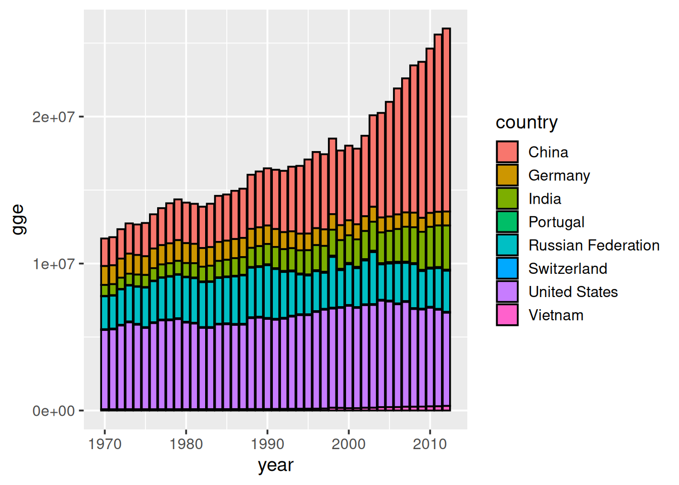
- Jahreszahl für x-Achse
Treibhausgasemissionen über die Zeit pro Kopf
ggplot(data = d_wb_countries) +
  geom_col(mapping = aes(x = year, y = gge / pop, fill = country))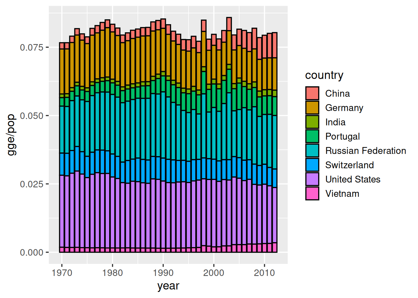
- Rechnen mit Merkmalen:
y = gge / pop
Treibhausgasemissionen anteilig
ggplot(data = d_wb_countries) +
  geom_col(mapping = aes(x = year, y = gge, fill = country), position = "fill")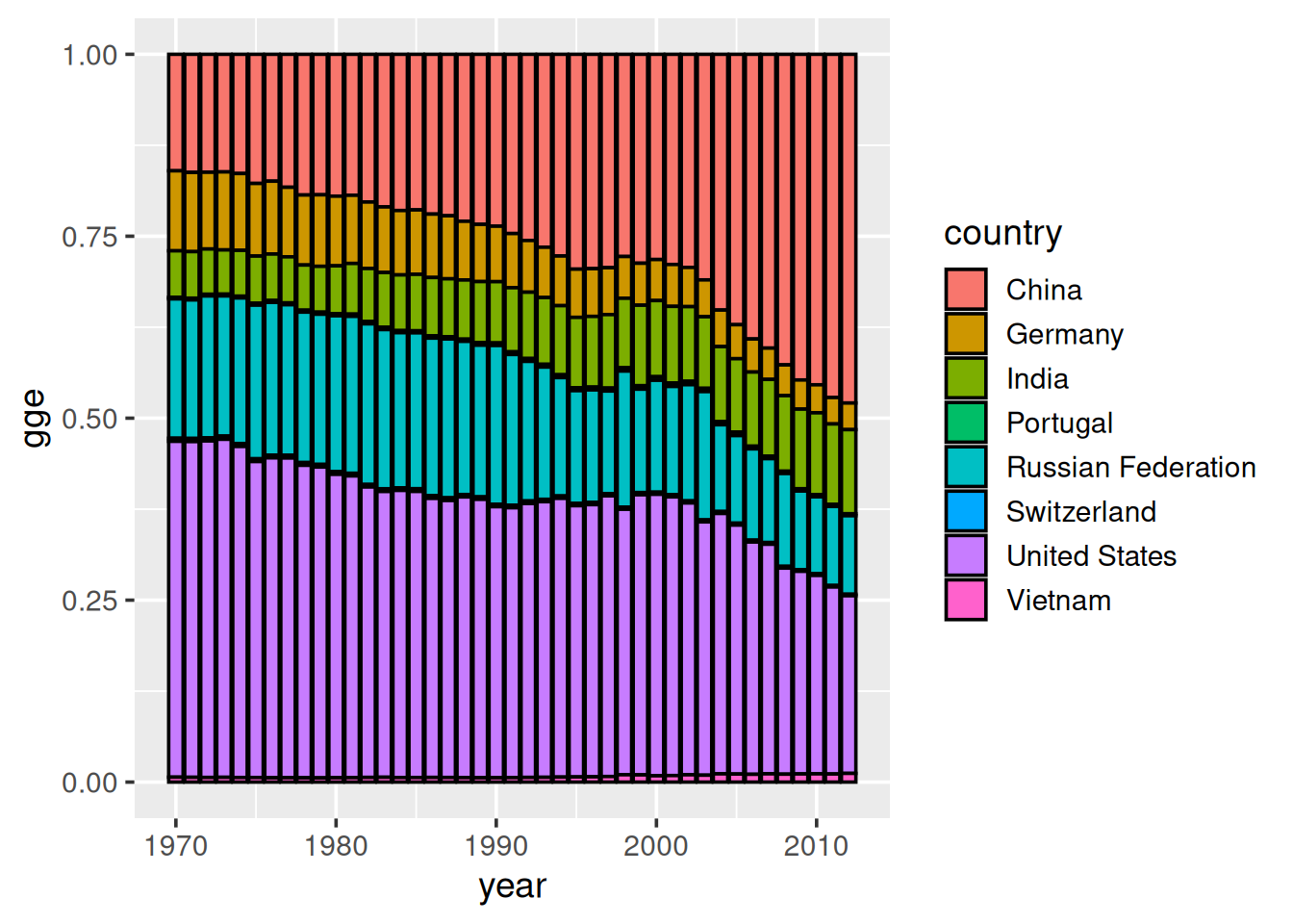
- Selbe Höhe für alle Balken mit
position = "fill"\(\rightarrow\) Anteile ablesbar
Ring- und Kreisdiagramme…
1. Schritt: Eine Säule mit Füllfarbe
ggplot(data = d_wb_countries_2012) +
  geom_col(mapping = aes(x = 0, y = pop, fill = country))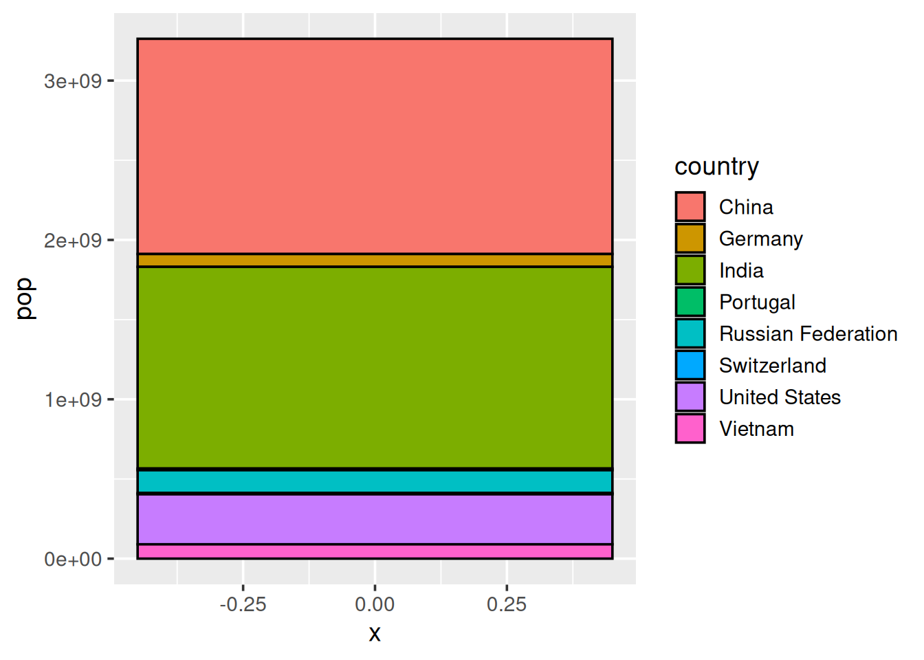
- x-Wert fest, Höhe nach Merkmal B, Füllfarbe nach Merkmal A
2. Schritt: Bereich auf der x-Achse
ggplot(data = d_wb_countries_2012) +
  geom_col(mapping = aes(x = 0, y = pop, fill = country)) +
  lims(x = c(-1.5, 0.5))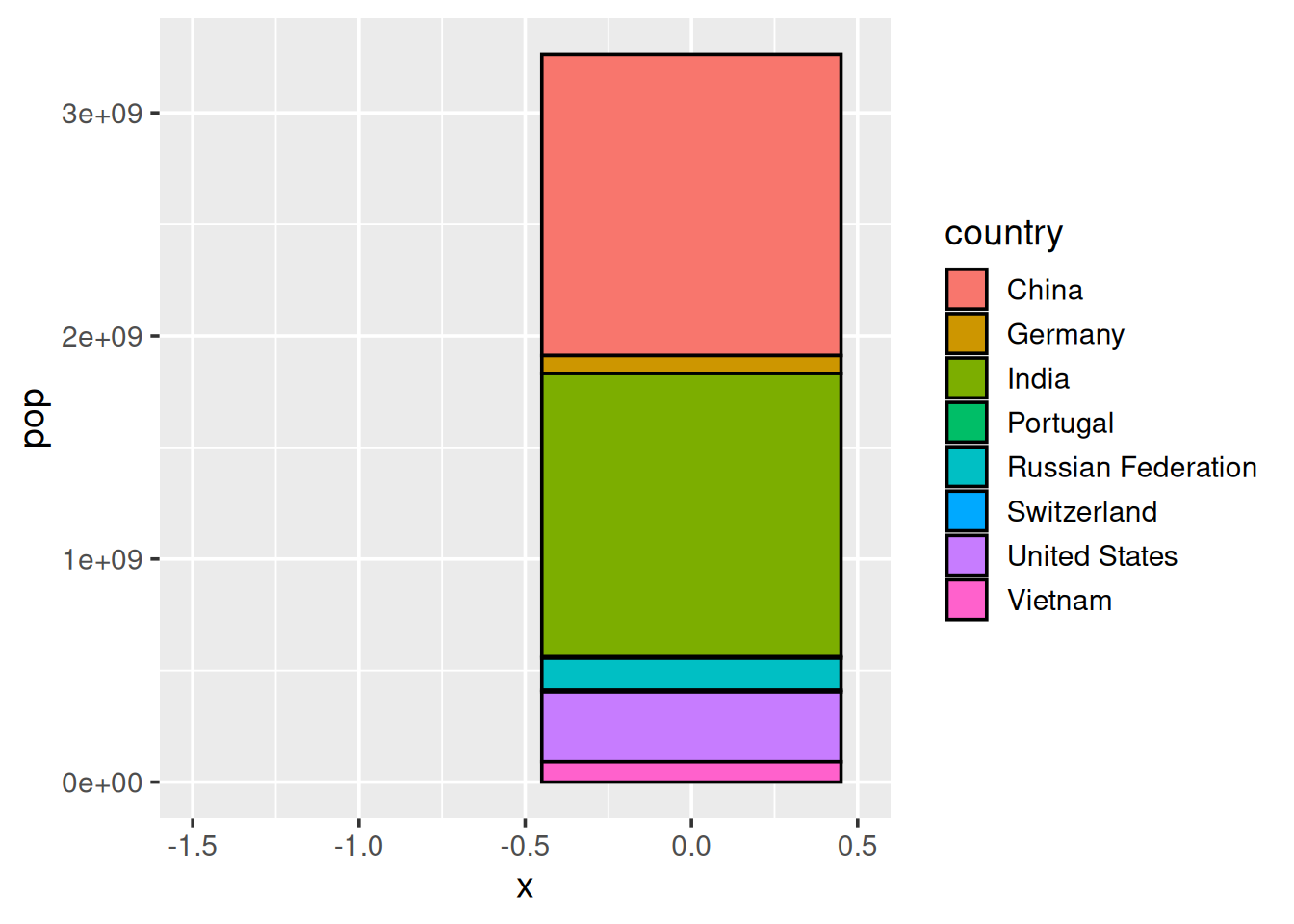
- Bereich auf der x-Achse mit
lims(x = c(-1.5, 0.5))
3. Schritt: Koordinatentransformation
ggplot(data = d_wb_countries_2012) +
  geom_col(mapping = aes(x = 0, y = pop, fill = country)) +
  lims(x = c(-1.5, 0.5)) +
  coord_polar(theta = "y")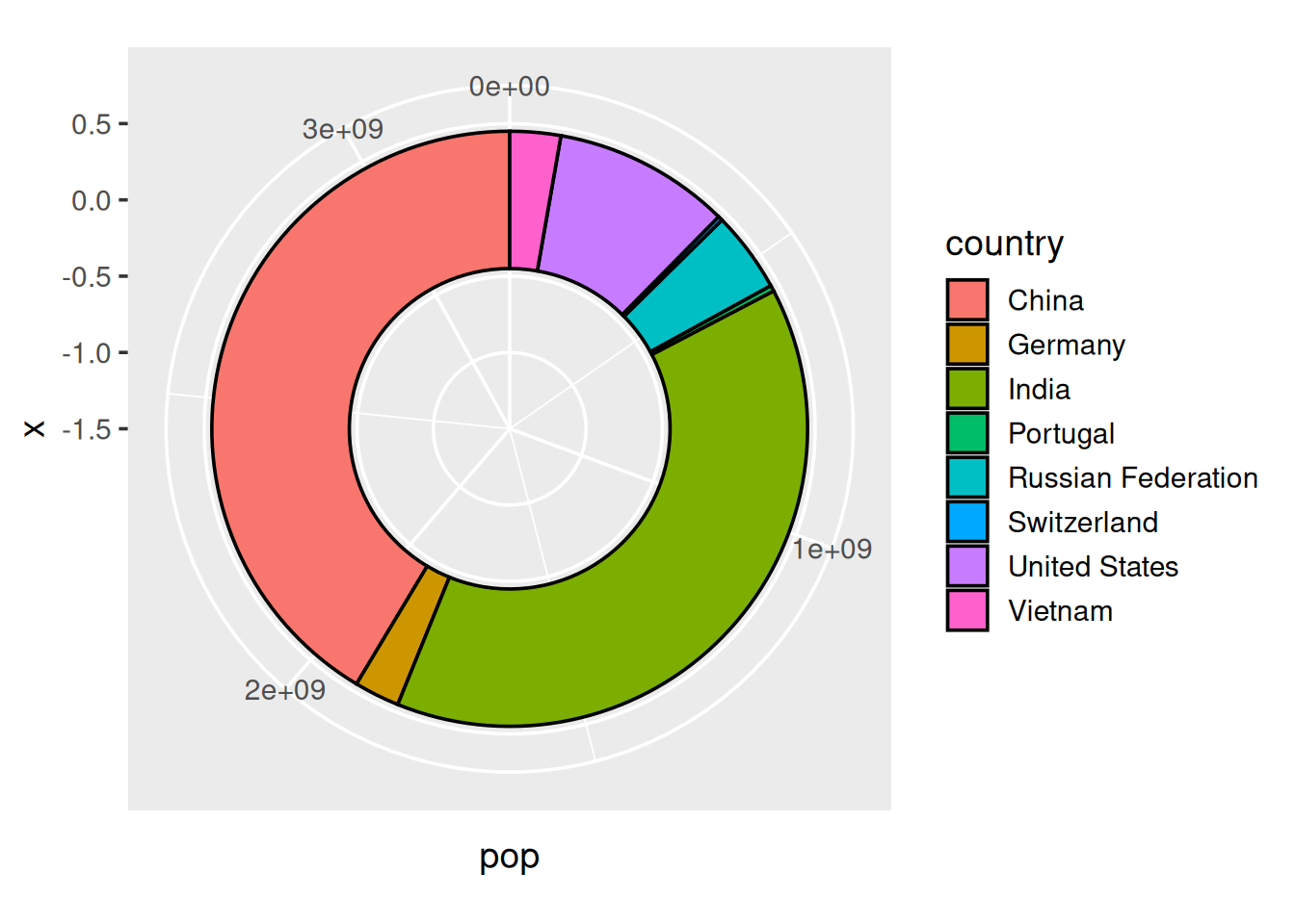
- y-Koordinate wird für den Winkel verwendet
Kreisdiagramm
ggplot(data = d_wb_countries_2012) +
  geom_col(mapping = aes(x = 0, y = pop, fill = country)) +
  coord_polar(theta = "y")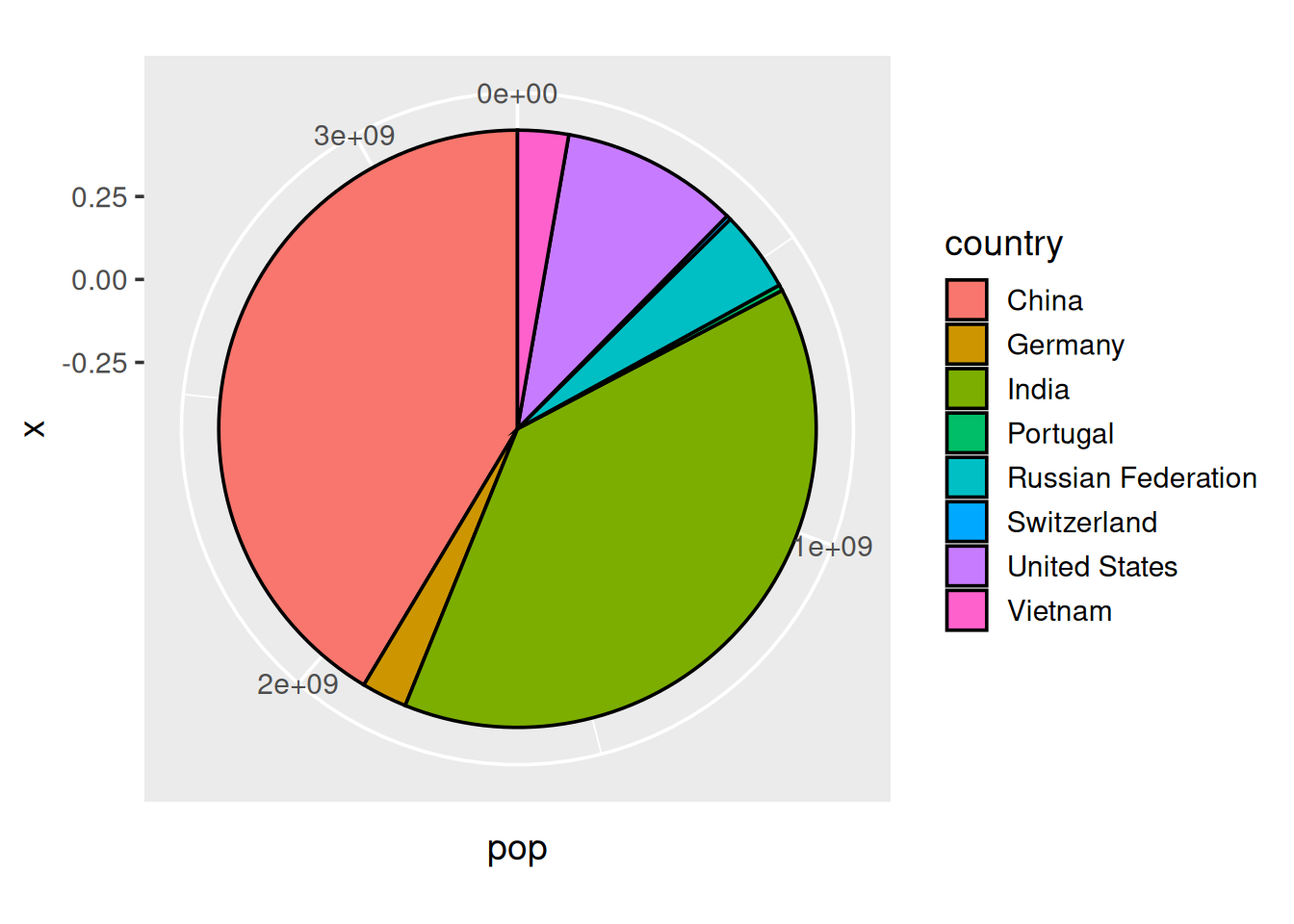
- Wie Ringdiagramm, aber kein Bereich für x-Werte vorgeben
Ohne Schnickschnack
ggplot(data = d_wb_countries_2012) +
  geom_col(mapping = aes(x = 0, y = pop, fill = country)) +
  coord_polar(theta = "y") +
  theme_void()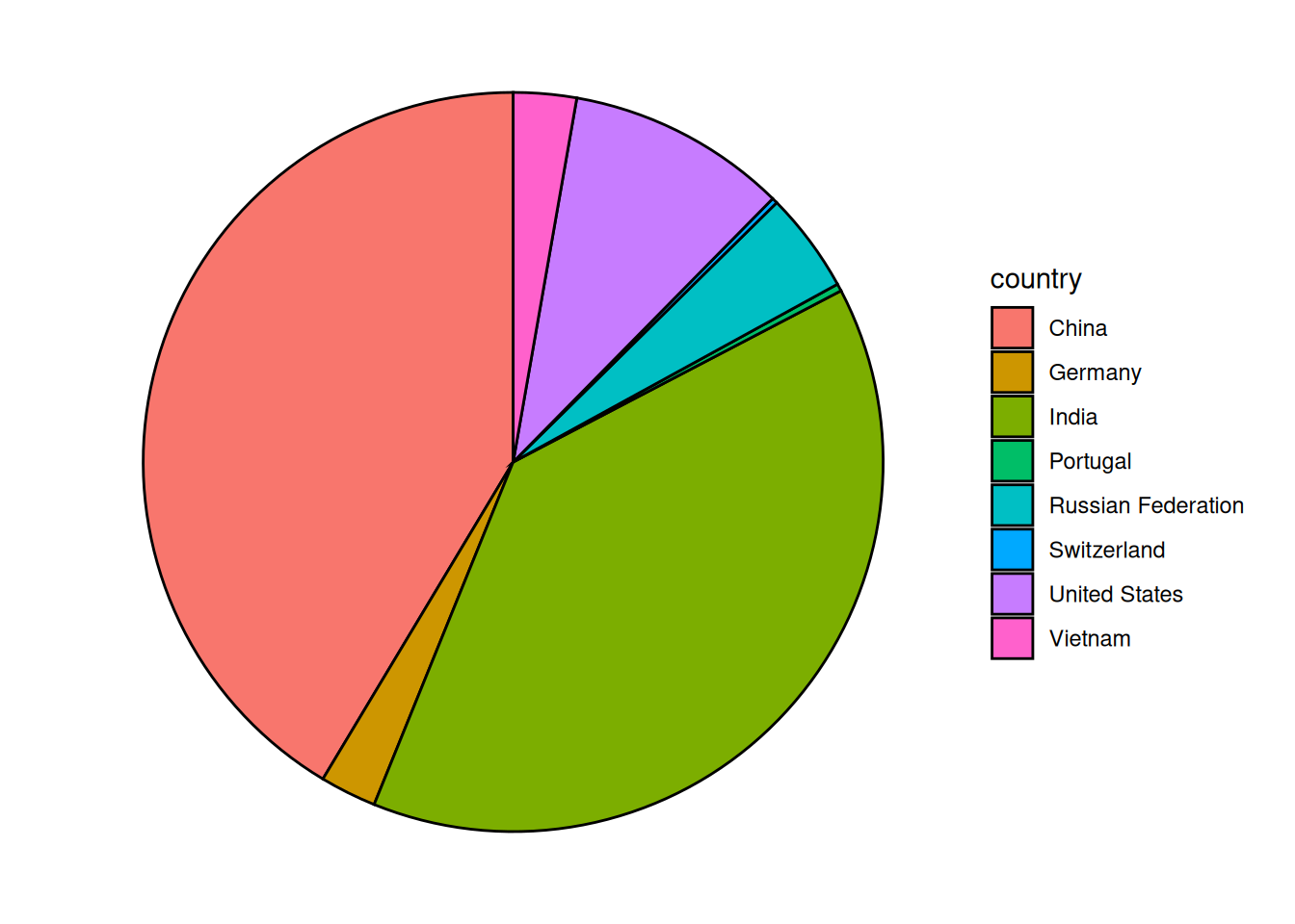
- Themes behandeln wir noch ausführlich
4.2 Häufigkeitsverteilungen mit geom_bar()
Wie geom_col() aber mit Zählen
Beispieldatensatz
d <- tibble(
  farbe = c("rot", "gruen", "blau", "gruen", "rot", "gruen")
)
Minimalbeispiel
ggplot(data = d) + geom_bar(mapping = aes(x = farbe))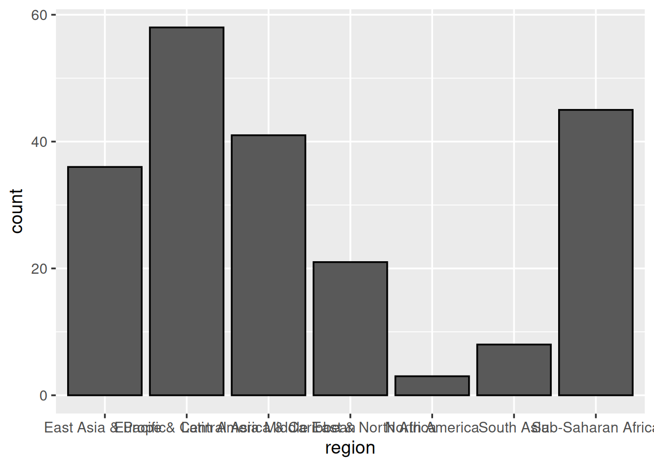
- Wie funktioniert das? Mit einer statistischen Transformation!
Statistische Transformation
![]()
Funktionsweise
- Daten werden vor dem Plotten transformiert
- Dabei wird eine neue Tabelle erzeugt
- Voreingestellte statistische Transformation für
geom_bar: Zählen - Transformierte Daten werden geplottet
Mit echten Daten…
Anzahl der Länder pro Region
ggplot(data = d_wb_2012) + geom_bar(mapping = aes(x = region))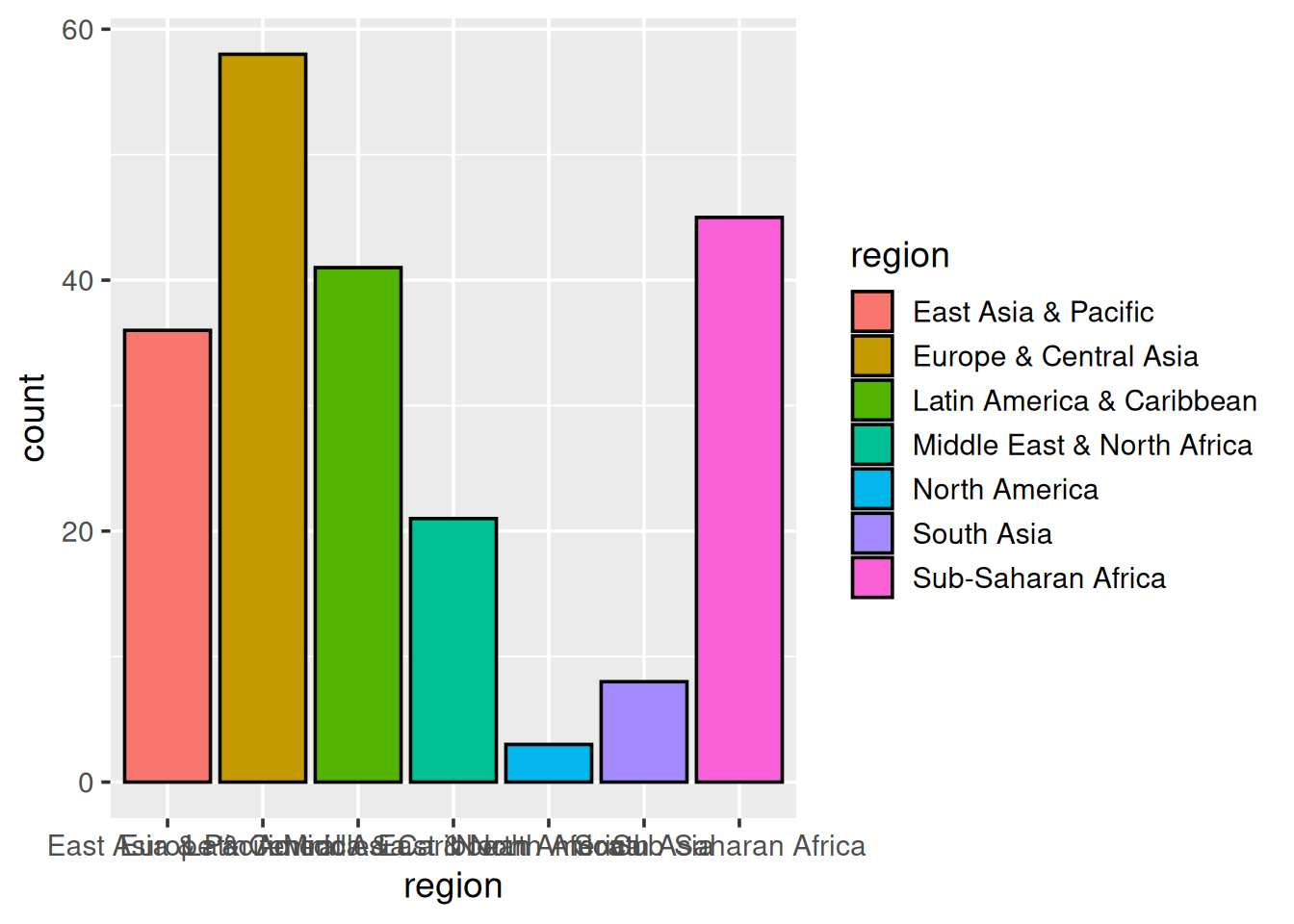
- Funktioniert, weil jedes Land genau einmal in
d_wb_2012vorkommt
Anzahl der Länder pro Region
ggplot(data = d_wb_2012) + geom_bar(mapping = aes(x = region, fill = region))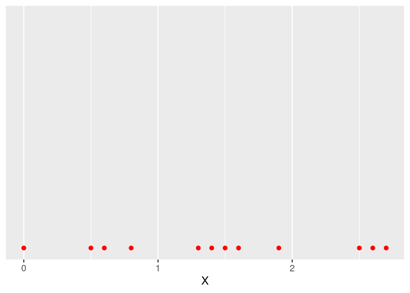
- Balken nach Region eingefärbt (redundant mit Achsenbeschriftung)
4.3 Histogramme mit geom_histogram()
Beispieldatensatz
d <- tibble(X = c(0, 0.5, 0.6, 0.8, 1.3, 1.4, 1.5, 1.6, 1.9, 2.5, 2.6, 2.7))

ggplot(data = d) + geom_point(mapping = aes(x = X), y = 0, color = "red")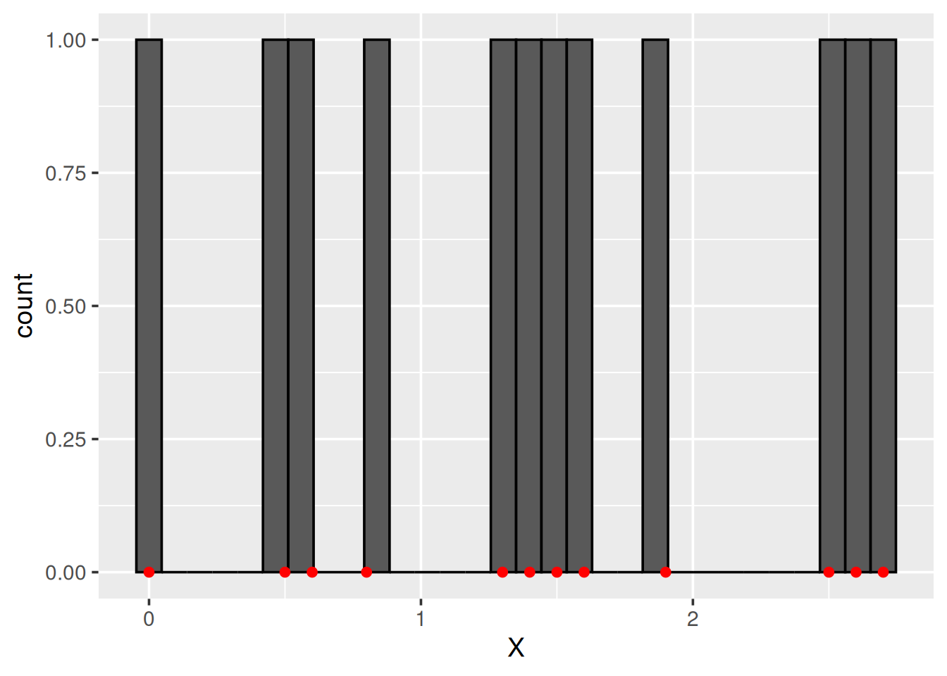
Histogramm
ggplot(data = d) +
  geom_histogram(mapping = aes(x = X)) +
  geom_point(mapping = aes(x = X), y = 0, color = "red")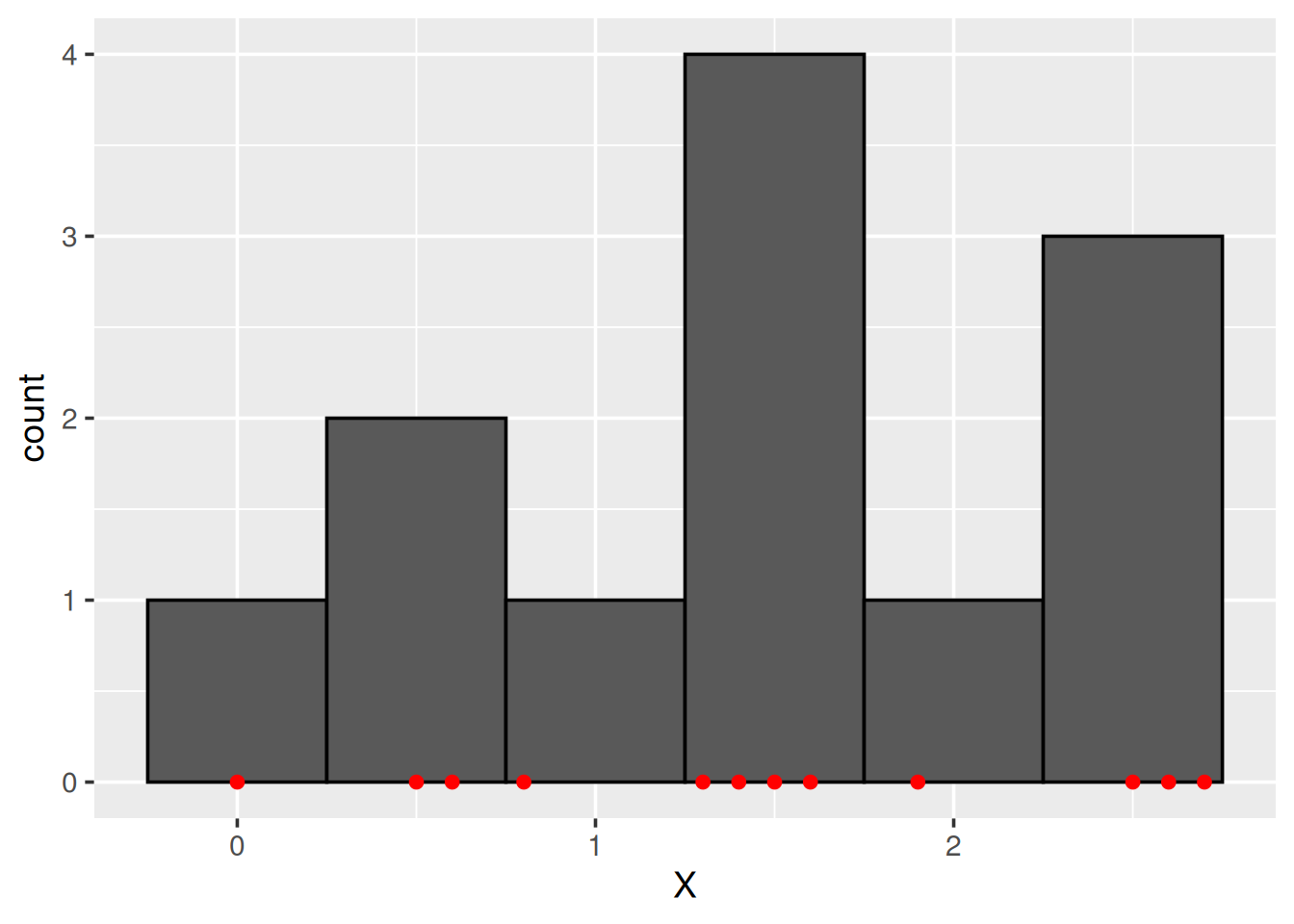
- Hinweis vom Programm: Voreinstellung nicht gut
Hilfetext zu geom_histogram
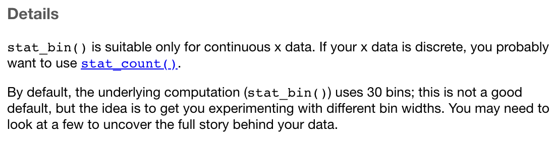
Histogramm anpassen 1/5
ggplot(data = d) +
  geom_histogram(mapping = aes(x = X), binwidth = 0.5) +
  geom_point(mapping = aes(x = X), y = 0, color = "red")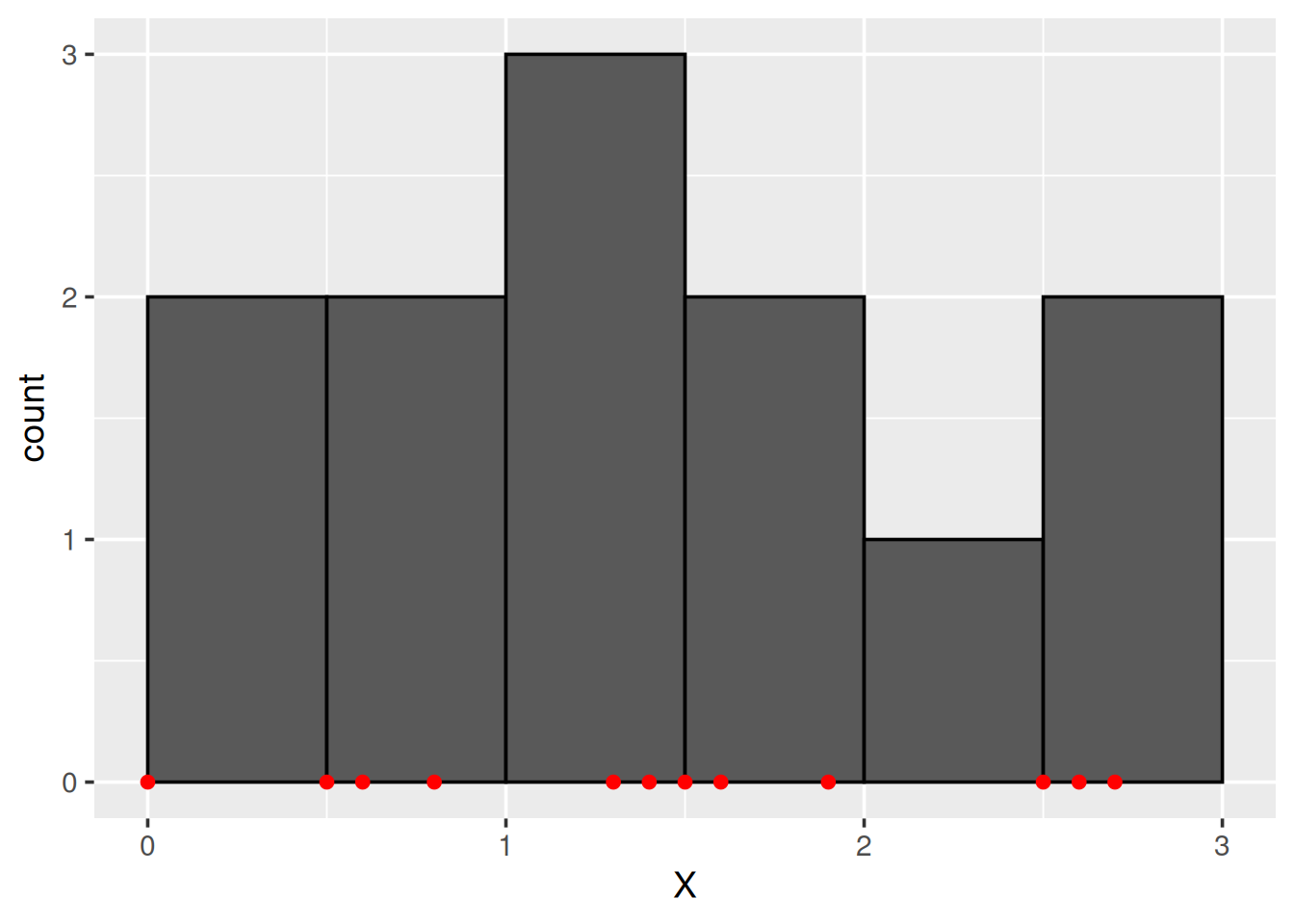
- Klassenbreite mit
binwidth
Histogramm anpassen 2/5
ggplot(data = d) +
  geom_histogram(mapping = aes(x = X), binwidth = 0.5, boundary = 0) +
  geom_point(mapping = aes(x = X), y = 0, color = "red")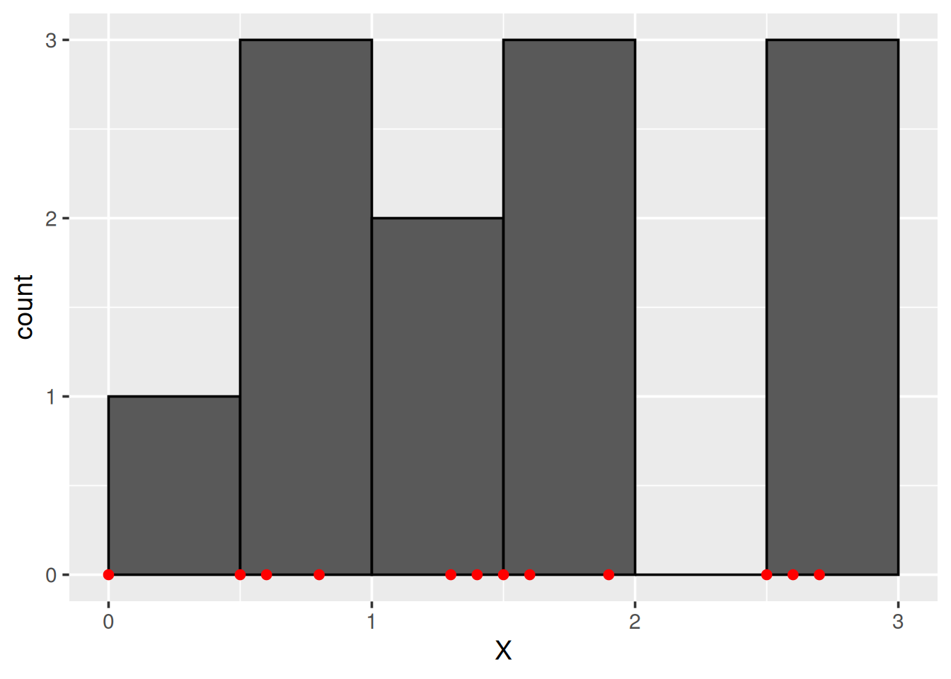
- Klassengrenze mit
boundary
Histogramm anpassen 3/5
ggplot(data = d) +
  geom_histogram(mapping = aes(x = X), binwidth = 0.5, boundary = 0, closed = "left") +
  geom_point(mapping = aes(x = X), y = 0, color = "red")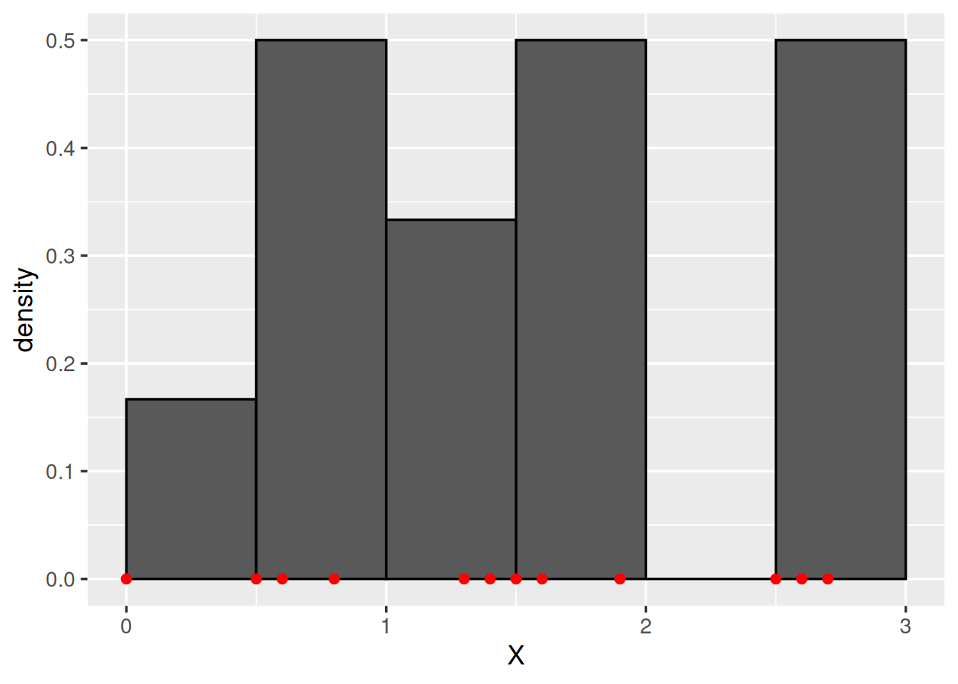
- Art der Intervalle (linksoffen, rechtsoffen) mit
closed
Histogramm anpassen 4/5
ggplot(data = d) +
  geom_histogram(mapping = aes(x = X, y = after_stat(density)), binwidth = 0.5, boundary = 0, closed = "left") +
  geom_point(mapping = aes(x = X), y = 0, color = "red")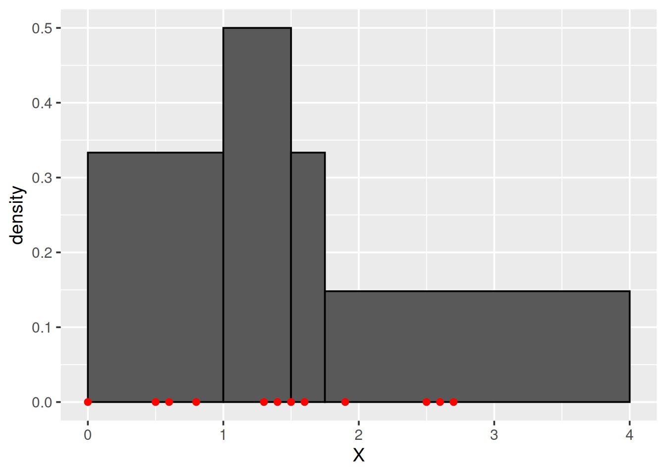
- Relative Häufigkeiten mit
y = after_stat(density)
Histogramm anpassen 5/5
ggplot(data = d) +
  geom_histogram(mapping = aes(x = X, y = after_stat(density)), breaks = c(0, 1, 1.5, 1.75, 4)) +
  geom_point(mapping = aes(x = X), y = 0, color = "red")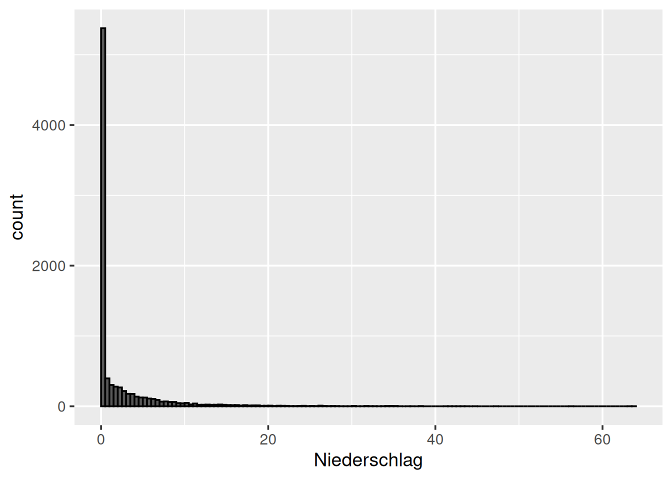
- Unterschiedliche Klassengrößen mit
breaks = c(...)
Mit echten Daten…
Niederschläge (Tag) in Bochum
ggplot(data = d_ns_bochum_tag) +
  geom_histogram(mapping = aes(x = Niederschlag), binwidth = 0.5, boundary = 0)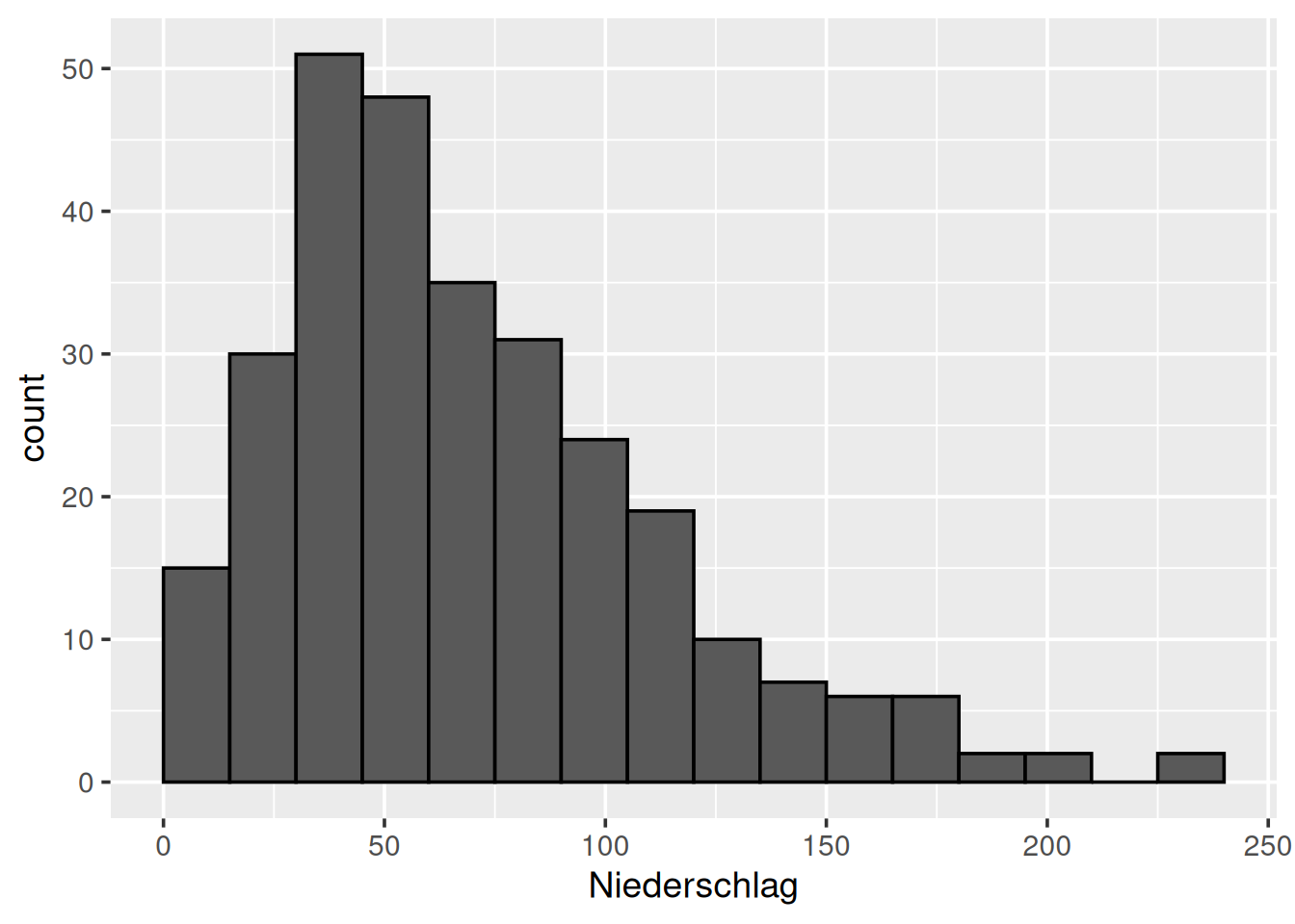
Niederschläge (Monat) in Bochum
ggplot(data = d_ns_bochum_monat) +
  geom_histogram(mapping = aes(x = Niederschlag), binwidth = 15, boundary = 0)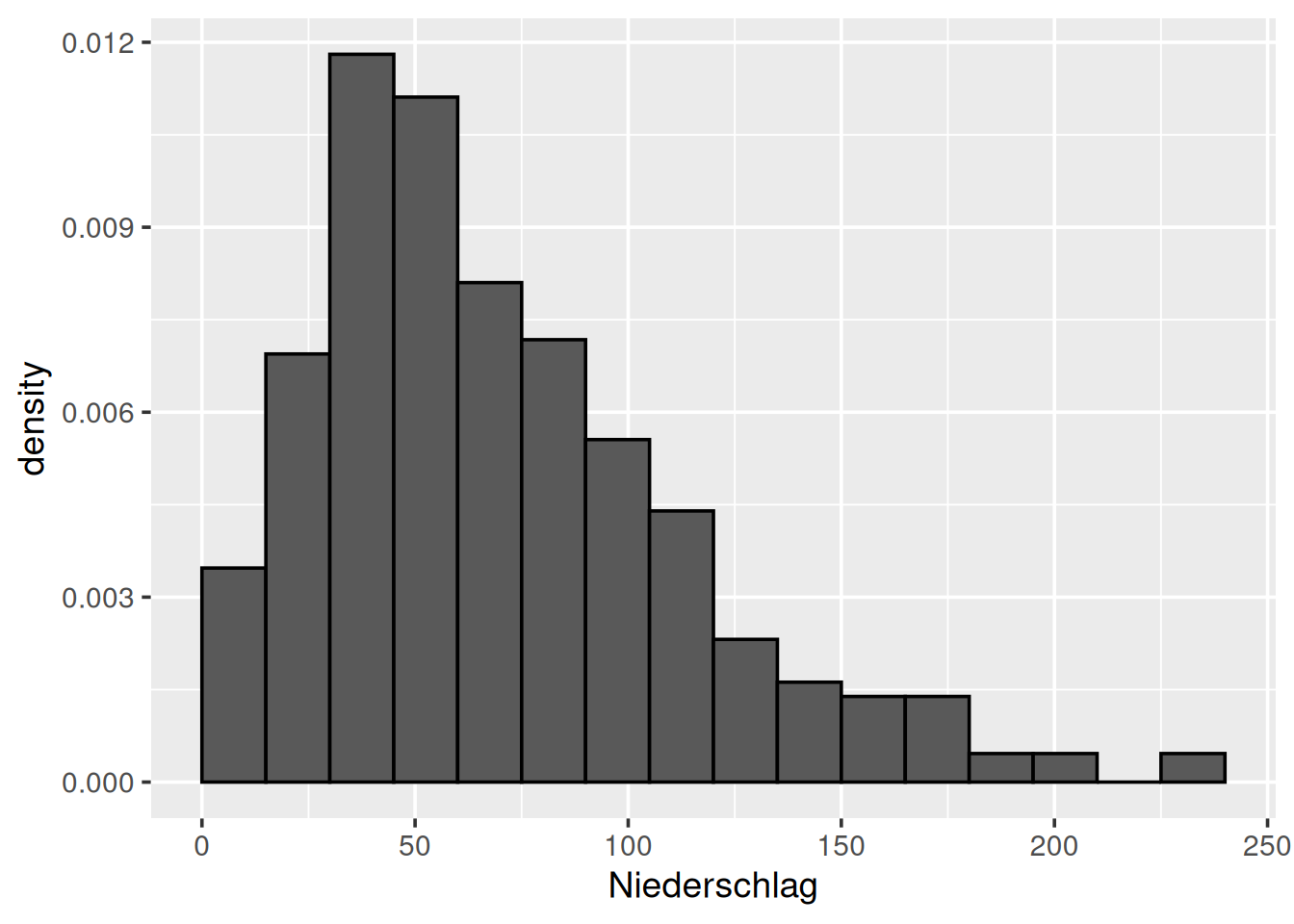
Niederschläge (Monat, relative Häufigkeit) in Bochum
ggplot(data = d_ns_bochum_monat) +
  geom_histogram(mapping = aes(x = Niederschlag, y = after_stat(density)), binwidth = 15, boundary = 0)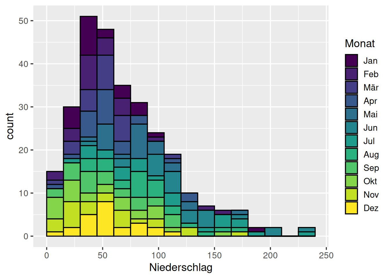
4.4 Verteilungsfunktionen mit geom_step() und Transformation
Minimalbeispiel geom_step()
ggplot(data = tibble(X = c(0, 1, 3), Y = c(2, 1, 3))) +
  geom_step(mapping = aes(x = X, y = Y)) +
  geom_point(mapping = aes(x = X, y = Y), color = "red")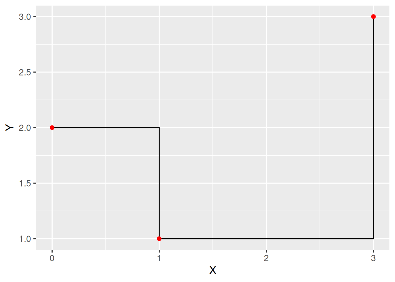
Beispieldaten
d <- tibble(
  X = c(0.0, 0.3, 0.2, 0.6, 0.3, 0.9, 1.0, 0.3, 0.6, 0.3),
  Y = c("a", "a", "a", "b", "b", "b", "a", "b", "a", "b")
)
ggplot(data = d) +
  geom_dotplot(mapping = aes(x = X, fill = Y), stackgroups = TRUE, dotsize = 0.5)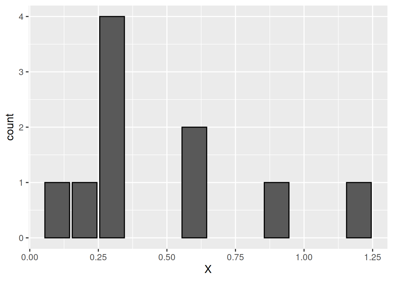
Empirische Verteilungsfunktion
ggplot(data = d) +
  geom_dotplot(mapping = aes(x = X), dotsize = 0.5) +
  geom_step(mapping = aes(x = X), stat = "ecdf")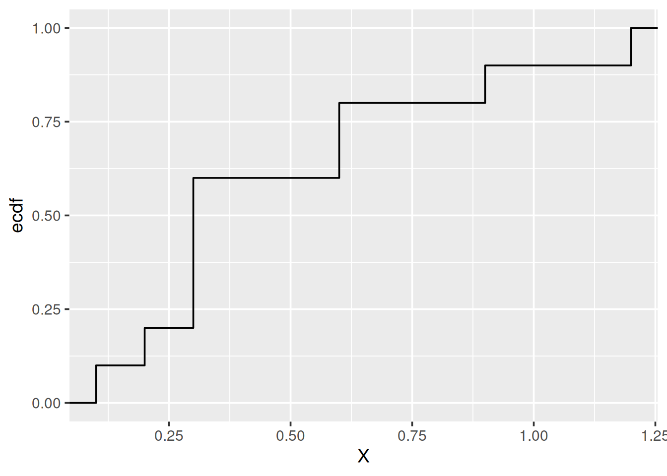
stat = "ecdf"meint Empirical Cumulative Densitiy Function
Empirische Verteilungsfunktion getrennt
ggplot(data = d) +
  geom_dotplot(mapping = aes(x = X, fill = Y), stackgroups = TRUE, dotsize = 0.5) +
  geom_step(mapping = aes(x = X, color = Y), stat = "ecdf")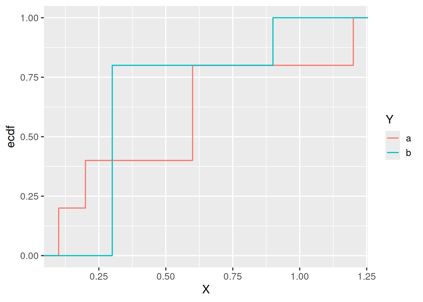
- Für jede Ausprägung von Merkmal
Yeine Kurve
Absolute kumulierte Häufigkeitsverteilung
ggplot(data = d) +
  geom_dotplot(mapping = aes(x = X), dotsize = 0.5) +
  geom_step(mapping = aes(x = X, y = nrow(d) * after_stat(y)), stat = "ecdf")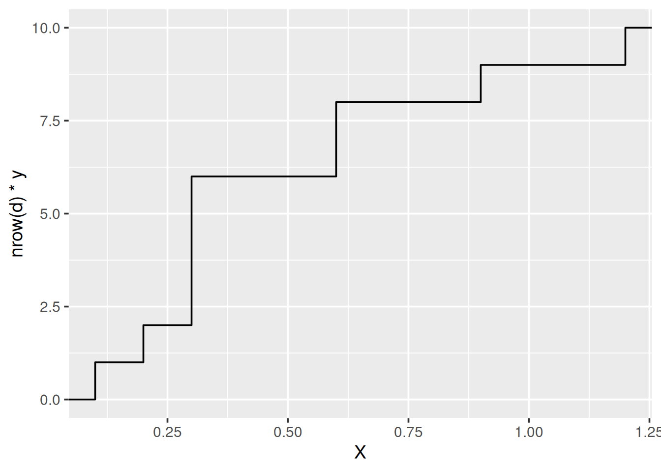
- In ggplot nicht vorgesehen und daher kompliziert
Mit echten Daten…
Monatliche Niederschläge
ggplot(data = d_ns_bochum_monat) +
  geom_step(mapping = aes(x = Niederschlag), stat = "ecdf")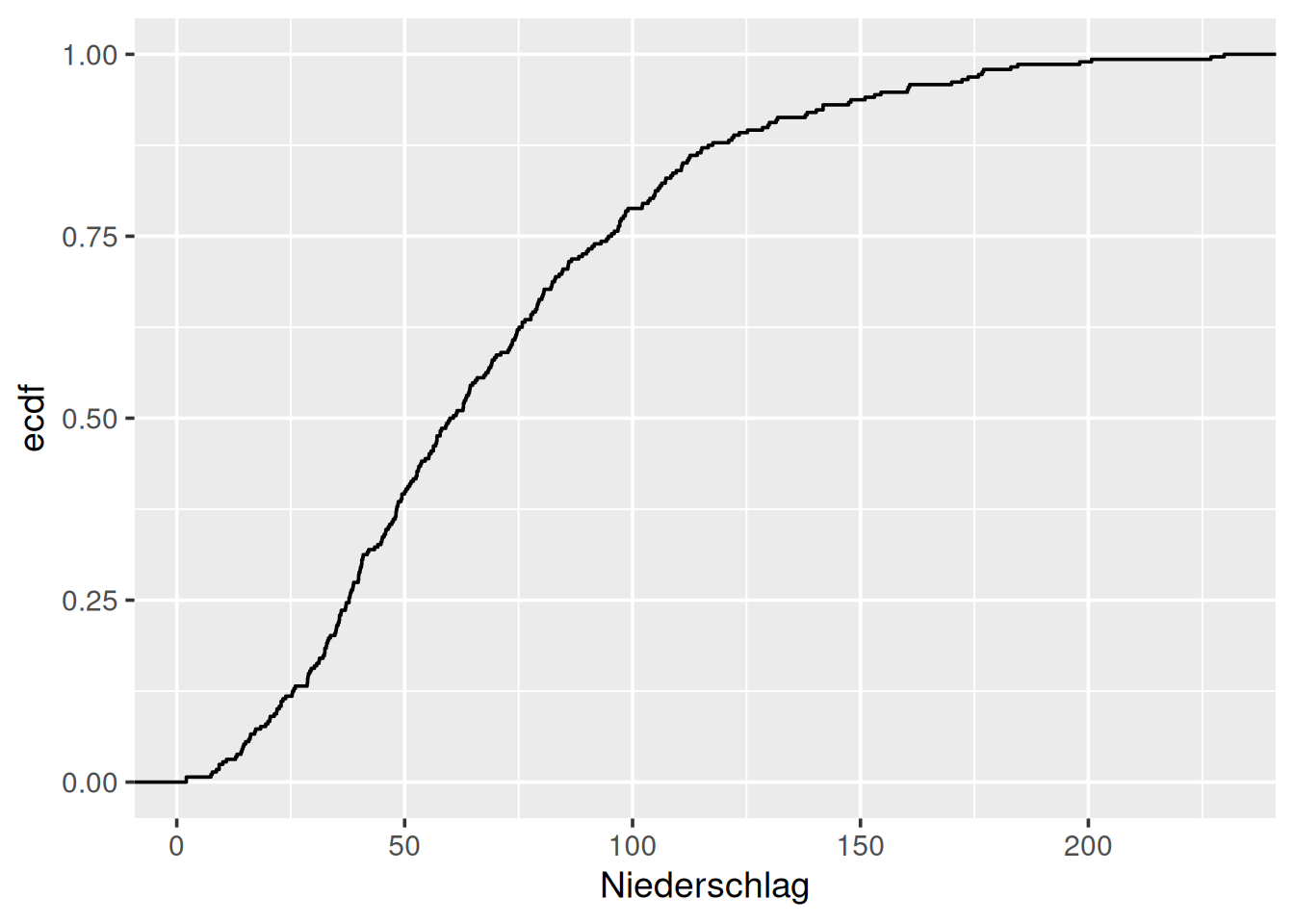
- So gut wie kein Monat ohne Regen
Tägliche Niederschläge
ggplot(data = d_ns_bochum_tag) +
  geom_step(mapping = aes(x = Niederschlag), stat = "ecdf")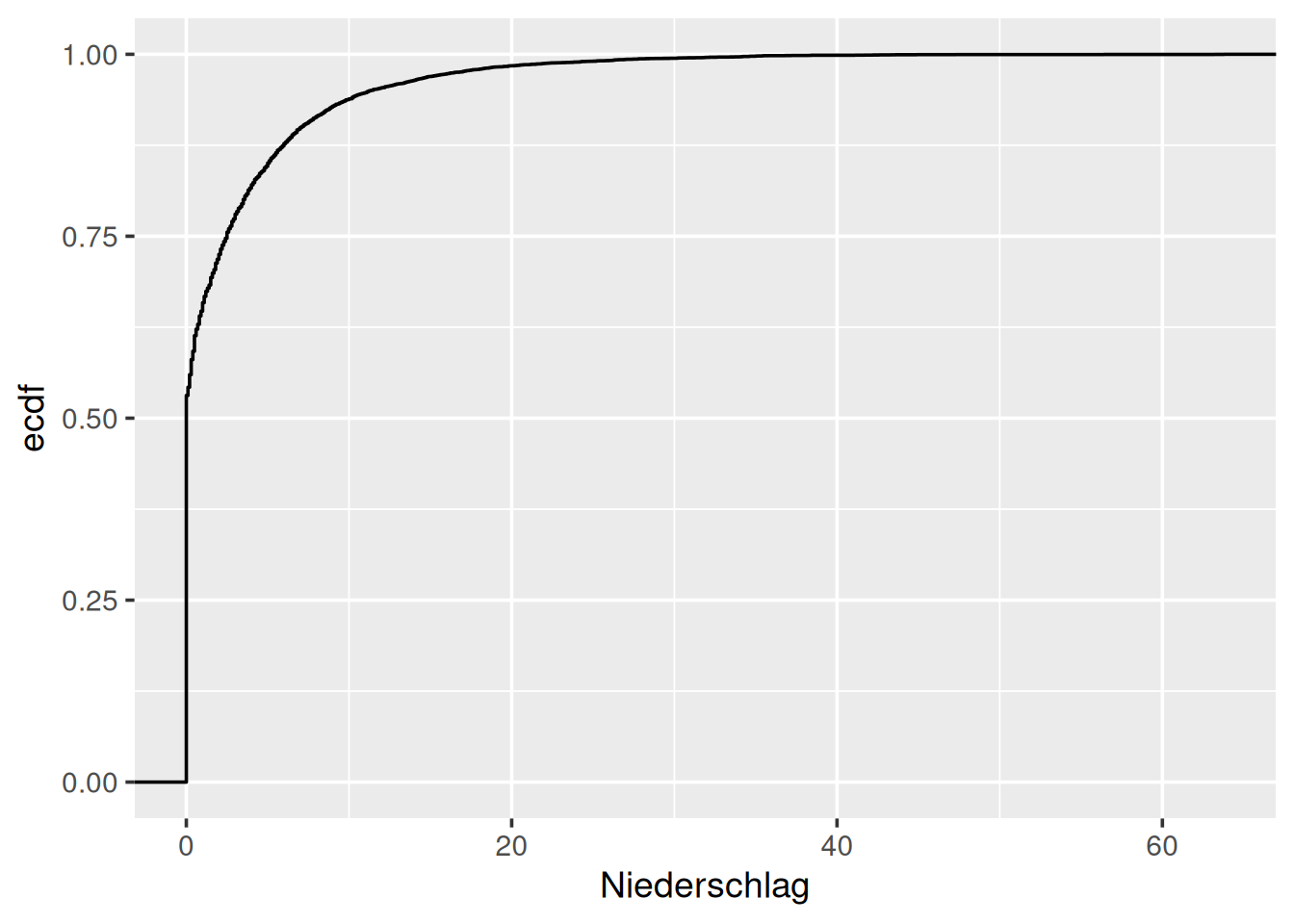
- Warum ganz anders als für die monatlichen Niederschläge?
4.5 Zusammenfassung
Werte darstellen mit geom_col()
ggplot(data = d) +
  geom_col(mapping = aes(x = <M>, y = <M>, fill = <M>, color = <M>), Argumente)
| Aesthetics | Beschreibung | Optional |
|---|---|---|
x |
Merkmal für x-Position | Nein |
y |
Merkmal für Höhe der Balken | Nein |
fill |
Merkmal für Füllfarbe | Ja |
color |
Merkmal für Linienfarbe | Ja |
| Argumente | Beschreibung |
|---|---|
position |
Gesamte y-Achse mit position = "fill" |
Balken nebeneinander mit position = "dodge" |
Zählen und darstellen mit geom_bar()
ggplot(data = d) +
  geom_bar(mapping = aes(x = <M>, fill = <M>, color = <M>), Argumente)
| Aesthetics | Beschreibung | Optional |
|---|---|---|
x |
Merkmal für x-Achse (wird gezählt) | Nein |
fill |
Füllfarbe | Ja |
color |
Linienfarbe | Ja |
| Argumente | Beschreibung |
|---|---|
position |
Gesamte y-Achse mit position = "fill" |
Balken nebeneinander mit position = "dodge" |
\(\rightarrow\) Wie geom_col aber ohne y
Histogramme mit geom_histogram()
ggplot(data = d) +
  geom_histogram(mapping = aes(x = <M>, y = after_stat(density), fill = <M>), Argumente)
| Aesthetics | Beschreibung | Optional |
|---|---|---|
x |
Merkmal, das gezählt werden soll | Nein |
y |
Relative Häufigkeiten mit y = after_stat(density)) |
Ja |
fill |
Merkmal für Füllfarbe | Ja |
| Argumente | Beschreibung |
|---|---|
bins |
Anzahl der Klassen |
binwidth |
Klassenbreite |
center |
Mitte einer Klasse |
boundary |
Grenze zwischen zwei Klassen |
breaks |
Klassengrenzen |
closed |
Intervalle geschlossen (“left” oder “right”) |
Empirische Verteilungsfunktion mit geom_step()
ggplot(data = d) +
  geom_step(mapping = aes(x = <M>, color = <M>), stat = "ecdf")
| Aesthetics | Beschreibung | Optional |
|---|---|---|
x |
Merkmal für empirische Verteilungsfunktion | Nein |
color |
Merkmal für Farbe | Ja |