ggplot(data = d_wb_2012) +
  geom_point(mapping = aes(x = gdp, y = gge, fill = region, size = pop), shape = 21) +
  scale_x_log10() + scale_y_log10() +
  labs(x = "Bruttoinlandsprodukt", y = "Treibhausgasemissionen", title = "Jahr 2012")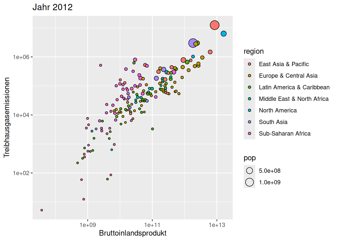
ggplot(data = d_wb_2012) +
geom_point(mapping = aes(x = gdp, y = gge, fill = region, size = pop), shape = 21) +
scale_x_log10() + scale_y_log10() +
labs(x = "Bruttoinlandsprodukt", y = "Treibhausgasemissionen", title = "Jahr 2012")


ggplot(data = <DATA>) +
  geom_<GEOM1>(mapping = aes(<AESTHETICS>), <ARGUMENTS>) +
  coord_<COORD>(<ARGUMENTS)> +
  facet_wrap(<ARGUMENTS>) +
  scale_<SCALE>(<ARGUMENTS>) +
  labs(<LABELS>) +
  theme(<THEME SETTINGS>)
→ Am Ende des Semesters werden Sie das verstehen!
d_wb_2012| Spalte | Deutsch | Englisch (Originaltitel) |
|---|---|---|
year |
Jahr | Year |
country |
Land | Country |
pop |
Bevölkerung | Population, total |
gge |
Treibhausgasemissionen kt CO2 äquivalent | Total greenhouse gas emissions kt of CO2 equivalent |
gdp |
Bruttoinlandsprodukt | GDP (current US$) |
region |
Region | Region |
ig |
Einkommensgruppe | Income group |
load("daten/data-lecture.Rdata")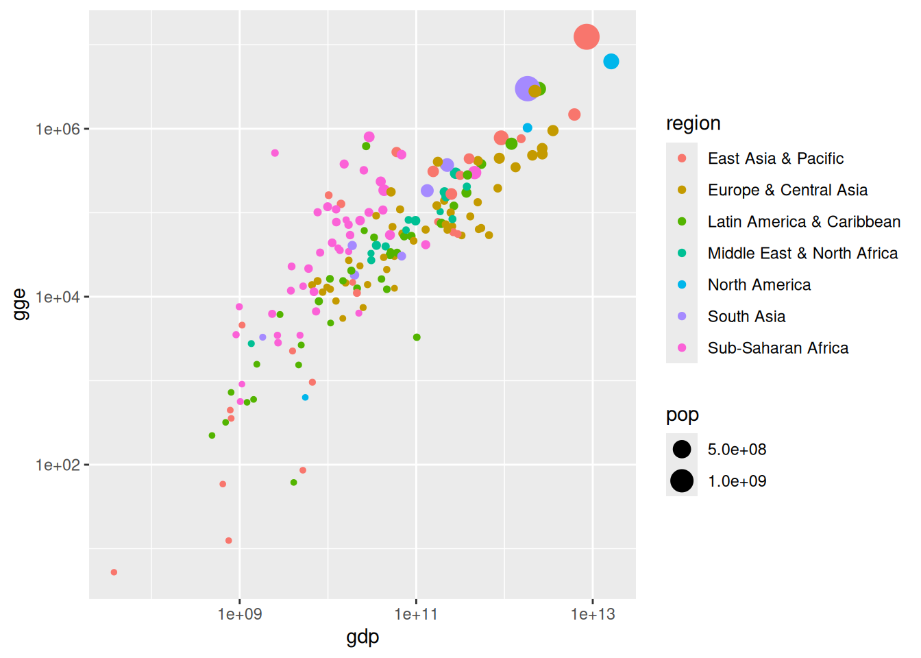
d_wb_2012ggplot(data = d_wb_2012) +
geom_point(mapping = aes(x = gdp, y = gge, fill = region, size = pop), shape = 21) +
scale_x_log10() + scale_y_log10() +
labs(x = "Bruttoinlandsprodukt", y = "Treibhausgasemissionen", title = "2012")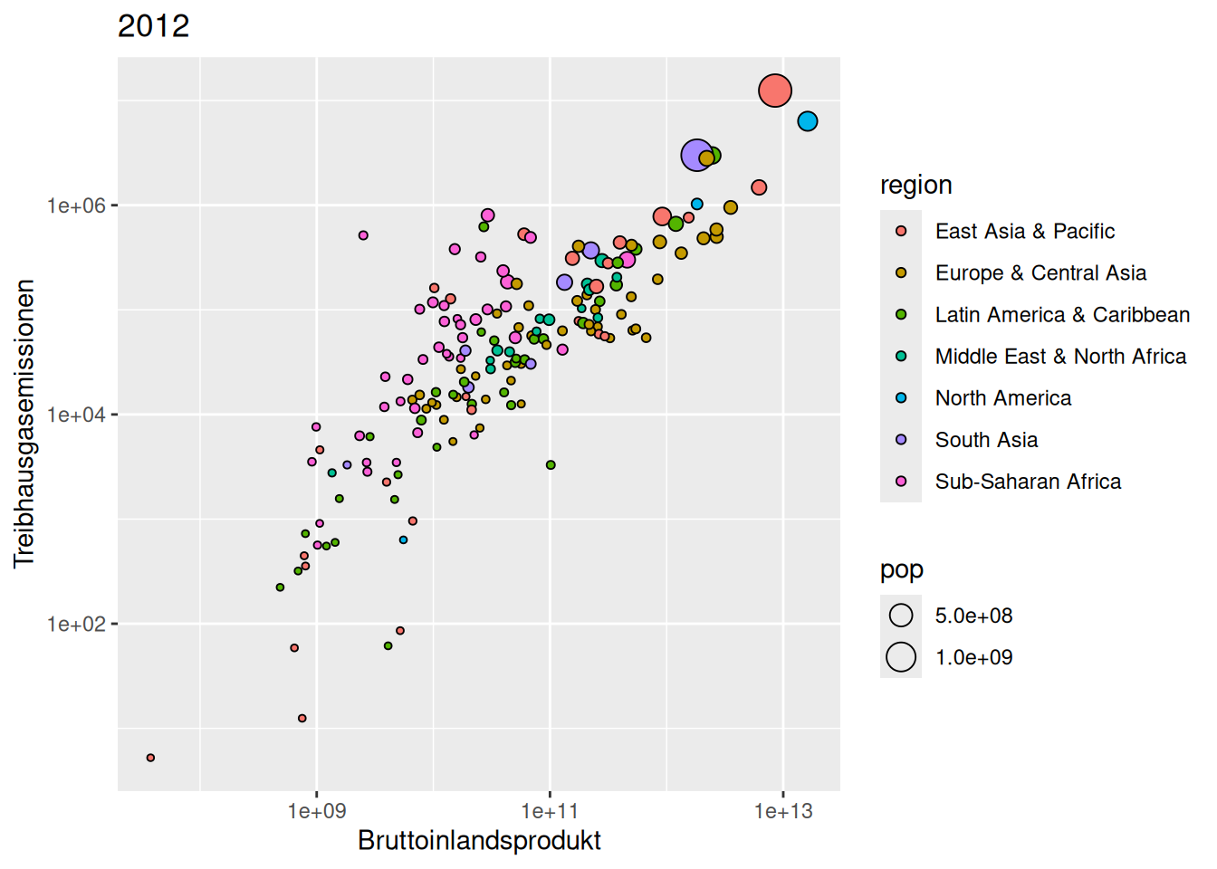
ggplot(data = d_wb_2012) +
  geom_point(mapping = aes(x = gdp, y = gge, fill = region, size = pop), shape = 21) +
  scale_x_log10() + scale_y_log10() +
labs(x = "Bruttoinlandsprodukt", y = "Treibhausgasemissionen", title = "2012")+ verbunden werdenggplot(...) erzeugt leere Zeichenfläche
geom_point(...) fügt Punkte (geometrische Objekte) hinzu

goem_point(mapping = aes(x = A, y = B, color = C, size = D))→ Visuelle Eigenschaften heißen in ggplot Aesthetics (AES)
d_bsp <- tibble(
  A = c(1, 3, 2),
  B = c(1, 2, 3),
  C = c("u", "v", "u"),
  D = c(5, 2, 4)
)ggplot(data = d_bsp) +
geom_point(mapping = aes(x = A, y = B, color = C, size = D))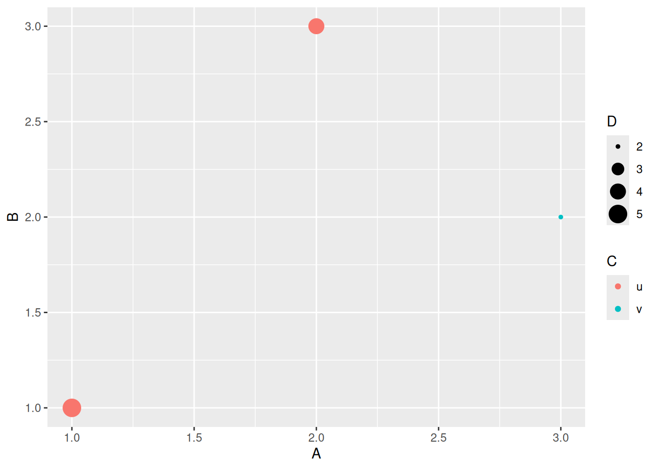

ggplot(data = d_wb_2012) +
  geom_point(mapping = aes(x = gdp, y = gge, color = region, size = pop))
ggplot(data = d_wb_2012) +
  geom_point(mapping = aes(x = gdp, y = gge, color = region, size = pop))
geom_point(...) sagt, dass Punkte geplottet werden sollenmapping definiert Zuordnung von Merkmalen auf visuelle Eigenschaftenaes(...) erzeugt. Hier:
gdp) und Emission (gge)region)pop)ggplot(data = d_wb_2012) +
geom_point(mapping = aes(x = gdp, y = gge, color = region, size = pop)) +
scale_x_log10() + scale_y_log10()