Räumliche Daten

Lukas Arnold

Simone Arnold

Florian Bagemihl

Matthias Baitsch

Marc Fehr

Franca Hollmann

Maik Poetzsch

Sebastian Seipel

2026-03-19

1 Einführung

Räumliche Daten

GIS Layer, Quelle: http//landportal.org

Viele Daten haben räumlichen Bezug
Klassische Anwendung von Geoinformationssystemen (GIS)
- Programme: ArcGIS (kommerziell) und QGIS (Open Source)
Verarbeitung räumlicher Daten schon seit langem auch in R
Gute Integration in ggplot2: Paket sf (simple feature)

Geographische Daten: Einzelne Punkte

Koordinatensystem mit Breiten- und Längengraden

Koordinaten eines Punktes mit Breitengrad (latitute) und Längengrad (longitude)
- Angaben im Winkelmaß
- Breitengrad ab Äquator (zwischen -90° und 90° oder mit Zusatz N/S)
- Längengrad ab Nullmeridian (zwischen -180° und 180° oder mit Zusatz O/W)
Schreibweise manchmal im Sexagesimalsystem (Winkelminuten und Sekunden)
- Koordinaten des Gipfels der Zugspitze: 47°25′16″N, 010°59′7″O
Die Erde ist keine Kugel
- Referenzellipsoid, häufig World Geodetic System 1984 (WGS 84)

GPS-Koordinaten Hochschule Bochum

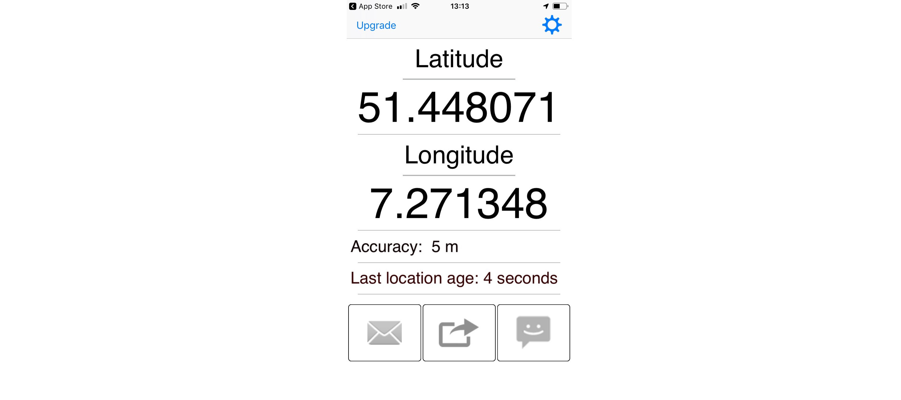
Hochschule Bochum liegt oberhalb vom 50. Breitengrad und etwas östlich vom 7. Längengrad

Mercator-Projektion 1/2

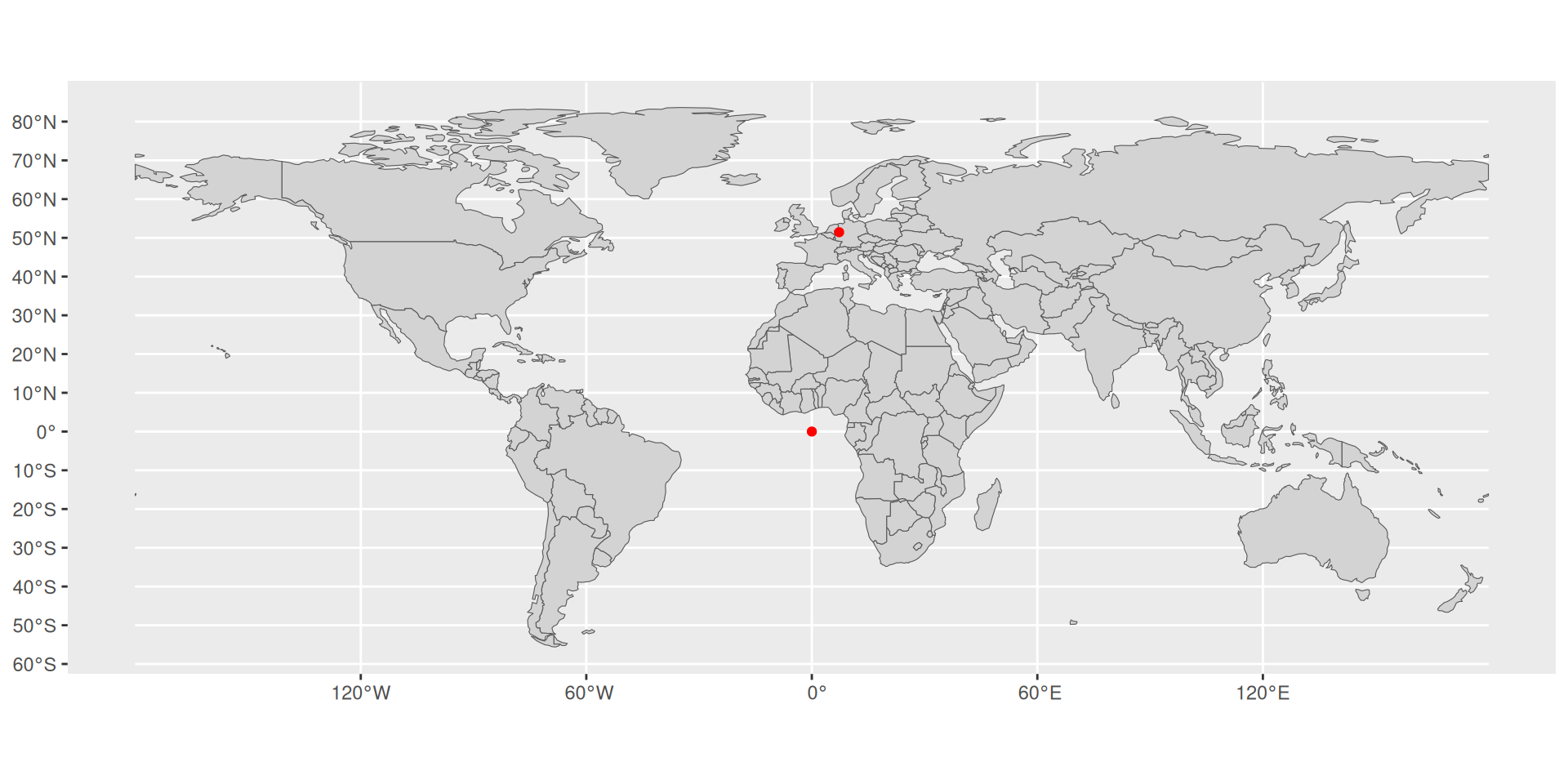
Breiten- und Längengrad in kartesischem Koordinatensystem
Problem: Länder am Äquator zu klein (oder umgekehrt)

Mercator-Projektion 2/2

Bild ist Link zum Film

Robinson-Projektion

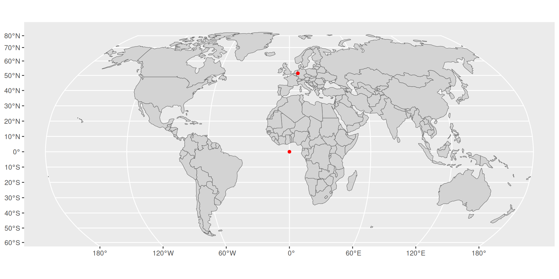
Breiten- und Längengrad in gekrümmtem Koordinatensystem
Keine Projektion im mathematischen Sinne

Lambertsche Azimutalprojektion

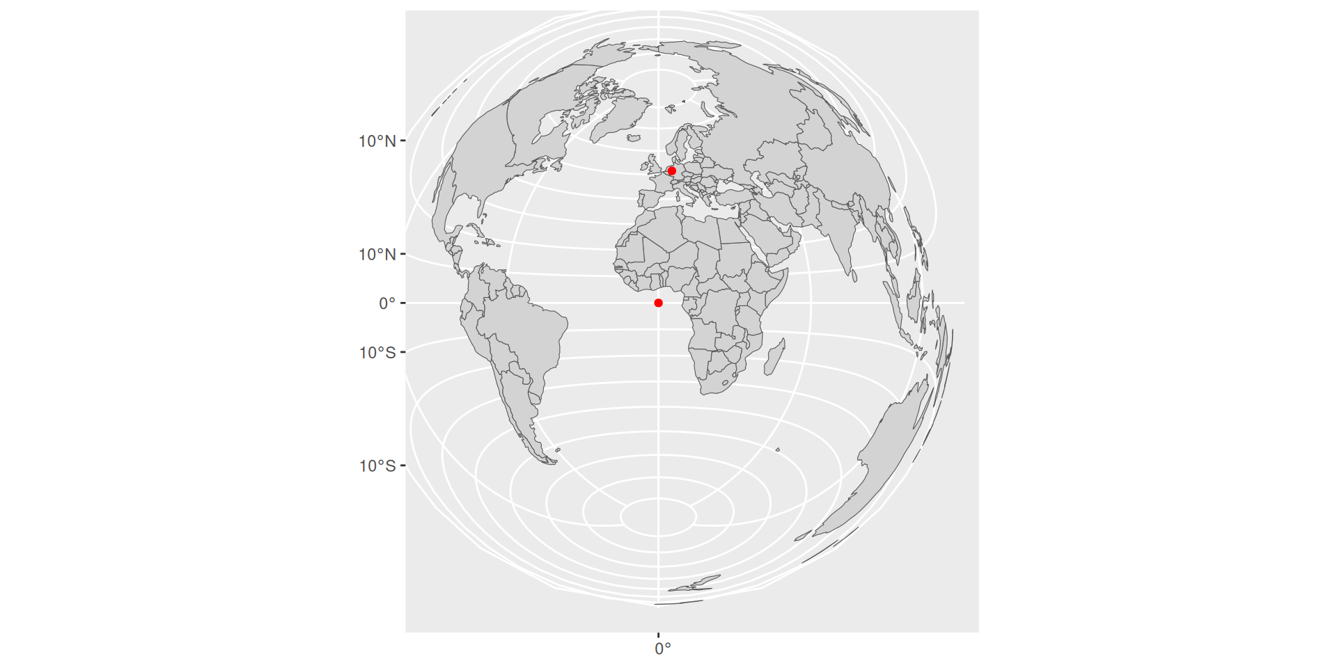
Flächen werden korrekt abgebildet
Weder winkel- noch längentreu

Geographische Daten: Geometrien

Simple Features

Offener Standard für geometrische Daten (ISO 19125-1:2004)
Entwickelt vom Open Geospatial Consortium (OGC)
Grundlage für viele GIS-Programme

R-Paket sf (Simple Features for R)

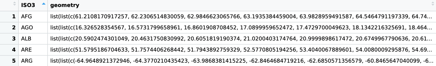
Paket sf: Simple Features in Dataframes

Beispiel oben: Dataframe der Weltkarte (Ausschnitt)
Ganz normaler Dataframe mit Spalten
- ISO3 (Ländercode)
- geometry (Geometrie eines Landes als Simple Feature)
Kann mit ggplot2 geplottet werden
Mehr Informationen hier

2 Weltkarte mit Natural Earth

Daten: Die Welt als Dataframe

d_world <- ne_countries() |>
  select(admin, adm0_a3, geometry) |>
  filter(adm0_a3 != "ATA")

Weltkarte mit ne_countries() als sf-Objekt (weitere Infos hier)
Benötigte Spalten mit select() auswählen
- ISO3-Codes der Länder (eindeutig)
- Geometrie
Die Antarktis interessiert uns nicht

Plot der Weltkarte

ggplot() +
  geom_sf(data = d_world)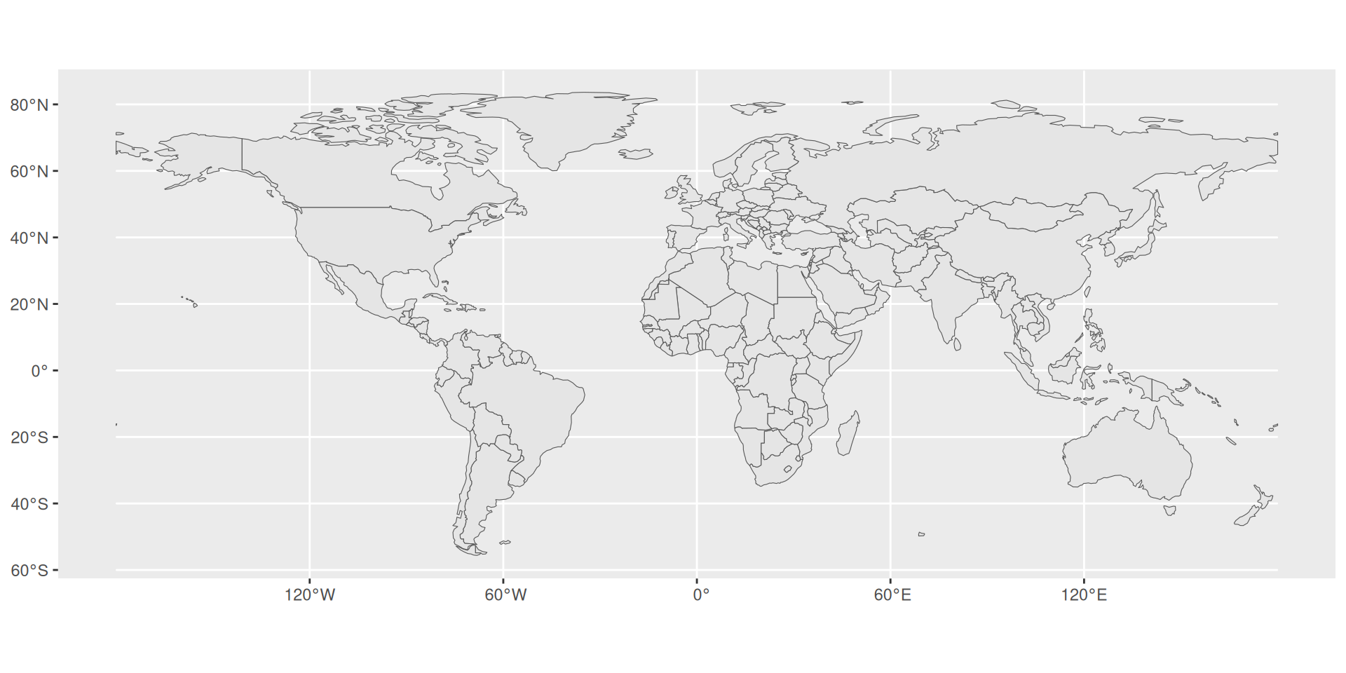

Plotten von sf Dataframes mit geom_sf()
Mapping für Geometrie ist eingebaut

3 Berechnung neuer Daten

Weltkarte mit Fläche der Länder 1/2

d_world_a <- d_world |>
  st_transform(crs = "EPSG:8857") |>
  mutate(area = as.numeric(st_area(geometry)) * 1e-6)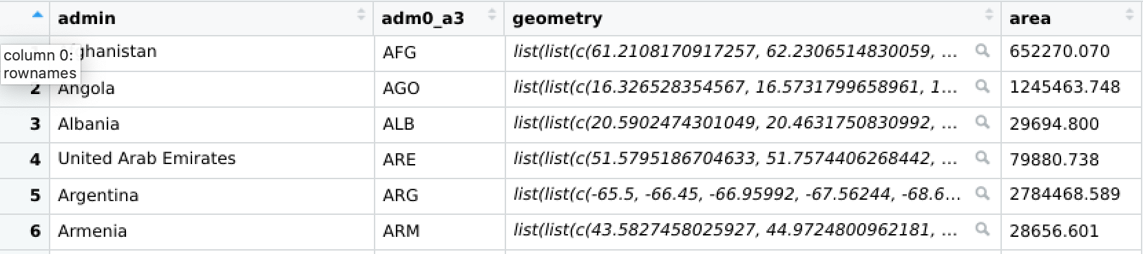

Flächentreue Projektion mit EPSG:8857
Berechnung der Flächen mit st_area()
Funktionen im sf-Paket beginnen mit st_ (🤯)
Einheiten entfernen mit as.numeric(), umrechnen in Quadratkilometer
Fläche Argentinien laut Wikipedia: 2.780.400 km²

Weltkarte mit Fläche der Länder 2/2

ggplot(data = d_world_a) +
  geom_sf(mapping = aes(fill = area)) +
  scale_fill_distiller(palette = 8, direction = 1)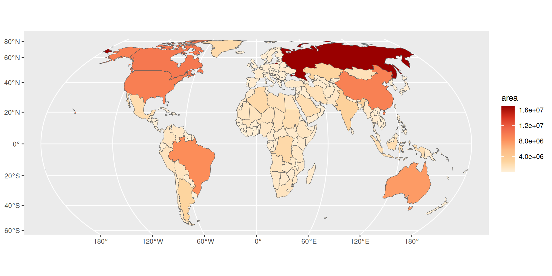

→ Choroplethenkarte, Flächenkartogramm oder Flächenwertstufenkarte

4 Kombination mit anderen Daten

Weltkarte mit der Lebenswerwartung

d_le <- wb_data(indicator = "SP.DYN.LE00.IN") |>
  select(adm0_a3 = iso3c, date, le = SP.DYN.LE00.IN) |>
  filter(!is.na(le)) |>
  group_by(adm0_a3) |>
  slice_max(date)

Dataframe mit wb_data() (Paket wbstats) herunterladen
- Indikator hier heraussuchen
Wichtige Merkmale auswählen und passend umbenennen
Für jedes Land den neuesten Wert heraussuchen

Dataframes miteinander verknüpfen

d_world_le <- d_world |>
  left_join(d_le, by = "adm0_a3")

Funktioniert, weil beide Dataframes eine Variable adm0_a3 haben
Natürlich nicht nur mit Daten von der Weltbank

Weltkarte mit Lebenserwartung

ggplot(data = d_world_le) +
  geom_sf(mapping = aes(fill = le)) +
  scale_fill_distiller(palette = "RdPu") + labs(fill = "Lebenserwartung")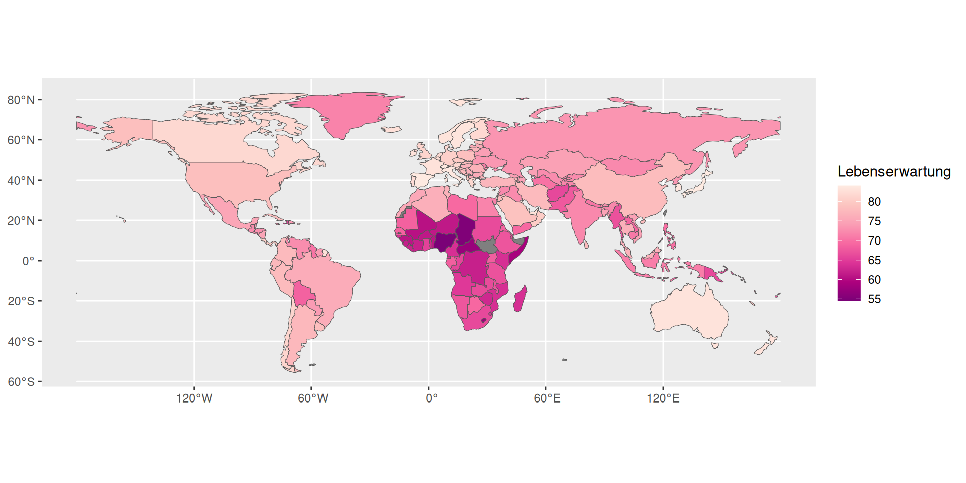

5 Werte zu einzelnen Koordinaten

Erste Möglichkeit: Mit `geom_point`

d_cities <- read_xlsx("daten/cities.xlsx")
ggplot() + geom_sf(data = d_world) +
  geom_point(data = d_cities, mapping = aes(x = long, y = lat, size = pop), color = "hotpink", show.legend = FALSE) + labs(x = NULL, y = NULL)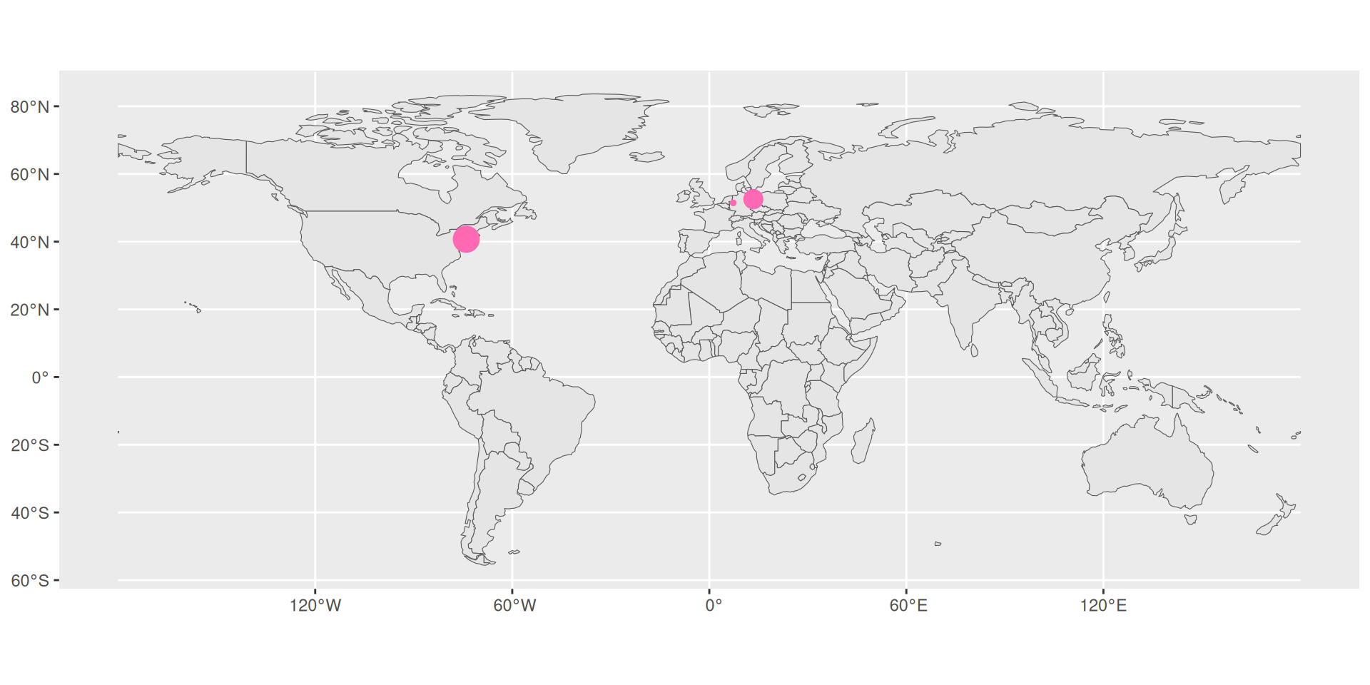

Geodaten zu Punkten mit Breitengrad und Längengrad
Darstellen mit geom_point() wie gehabt
Dataframe als Parameter zu geom
Klappt so einfach nur mit Mercator-Projektion

Besser: Dataframe konvertieren und `geom_sf`

d_cities_sf <- d_cities |> st_as_sf(coords = c("long", "lat"), crs = "+proj=longlat")
ggplot() + geom_sf(data = d_world) +
  geom_sf(data = d_cities_sf, mapping = aes(size = pop), color = "hotpink", show.legend = FALSE)

Dataframe in Simple Feature Objekt konvertieren mit st_as_sf
- Mit coords angeben in welchen Spalten die Koordinaten stehen
- Referenzkoordinatensystem angeben
Plotten mit geom_sf

6 Landesgrenzen mit `giscoR`

Landesgrenzen Bundesrepublik 1/2

d_de <- gisco_get_nuts(country = "Germany", nuts_level = 0, resolution = 10)
d_bl <- gisco_get_nuts(country = "Germany", nuts_level = 1, resolution = 10)
d_rb <- gisco_get_nuts(country = "Germany", nuts_level = 3, resolution = 10)

GISCO: Geografisches Informationssystem der EU-Kommission
Paket giscoR (R-Schnittstelle zu Daten der EU)
Datensatz laden mit gisco_get_nuts
- country Land
- nuts_level gibt Ebene an Staat/Bundesländer/Regierungsbezirke
- resolution Auflösung, siehe Dokumentation
- NUTS ist ein System zur Bezeichnung von Ländern

Landesgrenzen Bundesrepublik 2/2

ggplot() +
  geom_sf(data = d_rb, mapping = aes(fill = NUTS_NAME), linewidth = 0.1, show.legend = FALSE) +
  geom_sf(data = d_bl, fill = NA, linewidth = 0.5, color = "white") +
  geom_sf(data = d_de, fill = NA, linewidth = 0.75, color = "black") +
  theme_void()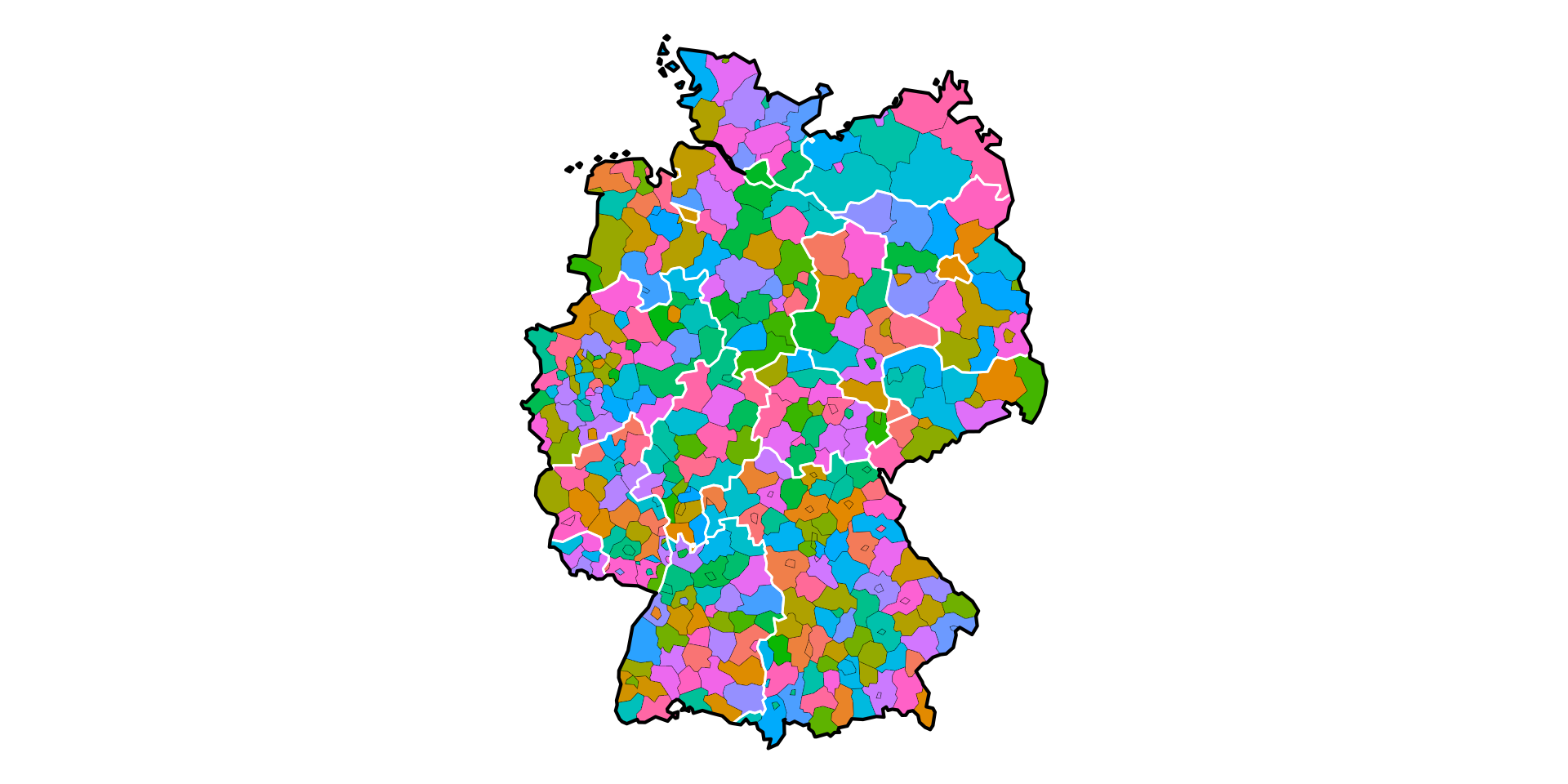

7 Open Street Map

Über Open Street Map

Freie Alternative zu Google Maps
Zugriff auf Daten aus eigenen Programmen
SEHR umfangreich aber nicht ganz einfach zu nutzen
In R mit Paket osmdata (https://github.com/ropensci/osmdata)

Straßen in Bochum 1/2

q <- opq(getbb("Bochum, Germany"))
s1 <- add_osm_feature(q, key = "highway", value = "motorway") |> osmdata_sf()

Bereich festlegen mit getbb (bb steht für Bounding Box)
Anfrage q erzeugen mit opq
Objekte zu Anfrage hinzufügen mit add_osm_feature
- key ist die Kategorie
- value sagt was genau gemeint ist
- Erläuterung hier
Mit osmdata_sf zur Verwendung mit SF aufbereiten
- Objekt enthält osm_points, osm_lines, osm_polygons, …
- Dies sind die eigentlichen SF-Dataframes

Straßen in Bochum 2/2

ggplot() +
  geom_sf(data = s1$osm_lines)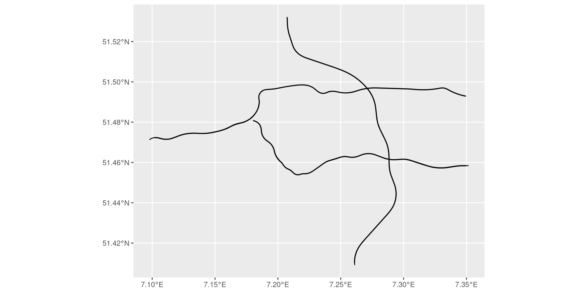

Mit $osm_lines die Linien heraussuchen

Karte von Bochum 1/3

if (!file.exists("daten/strassen-bochum.RData")) {
  q  <- opq(getbb("Bochum, Germany"))
  s1 <- add_osm_feature(q, key = "highway", value = c("motorway", "primary", "motorway_link", "primary_link")) |> osmdata_sf()
  s2 <- add_osm_feature(q, key = "highway", value = c("secondary", "tertiary", "secondary_link", "tertiary_link")) |> osmdata_sf()
  s3 <- add_osm_feature(q, key = "highway", value = c("unclassified", "residential")) |> osmdata_sf()
  f1 <- add_osm_feature(q, key = "waterway", value = "river") |> osmdata_sf()
  u1 <- add_osm_feature(q, key = "amenity", value = "university") |> osmdata_sf()
  save(s1, s2, s3, f1, u1, file = "daten/strassen-bochum.RData")
} else {
  load(file = "daten/strassen-bochum.RData")
}

Mit c mehrere Objekte aus einer Kategorie kombinieren
Daten teilweise recht umfangreich, Download kann dauern oder auch zu Abbrüchen oder Fehlermeldungen führen
Daher: Daten einmal herunterladen, auf Festplatte speichern und ab dann nur noch einlesen

Karte von Bochum 2/3

p <- ggplot() +
  geom_sf(data = u1$osm_polygons, color = "orange", linewidth = 0.35) +
  geom_sf(data = f1$osm_lines, color = "steelblue", linewidth = 0.35) +
  geom_sf(data = s3$osm_lines, color = "light gray", linewidth = 0.15) +
  geom_sf(data = s2$osm_lines, color = "dark gray", linewidth = 0.25) +
  geom_sf(data = s1$osm_lines, color = "black", linewidth = 0.35) +
  coord_sf(xlim = c(7.1, 7.3), ylim = c(51.41, 51.52)) +
  theme_void()

Plot in Variable p speichern und auf nächster Folie ausgeben

Karte von Bochum 3/3

Bundesautobahnen 1/2

if (!file.exists("daten/bab.RData")) {
  bab_raw <- opq(bbox = getbb("Deutschland", featuretype = "country")) |>
    add_osm_feature(key = "highway", value = "motorway") |>
    osmdata_sf()
  d_bab <- bab_raw$osm_lines |>
    st_filter(d_de, .predicate = st_within) |>
    drop_na(ref) |>
    group_by(ref) |>
    summarise() |>
    st_simplify(dTolerance = 100)
  save(d_bab, file = "daten/bab.RData")
} else {
  load(file = "daten/bab.RData")
}

Daten wieder zwischenspeichern (siehe oben)
Aufbereiten der Daten (auswählen, zusammenfassen und vereinfachen)

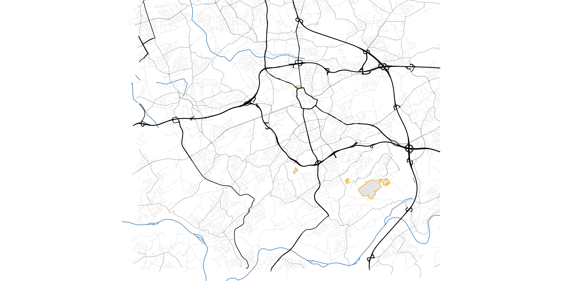
Bundesautobahnen 2/2

ggplot() +
  geom_sf(data = d_bl, linewidth = 0.25) +
  geom_sf(data = d_de, fill = NA, linewidth = 0.5) +
  geom_sf(data = d_bab, mapping = aes(color = ref), linewidth = 0.35, show.legend = FALSE) +
  theme_void()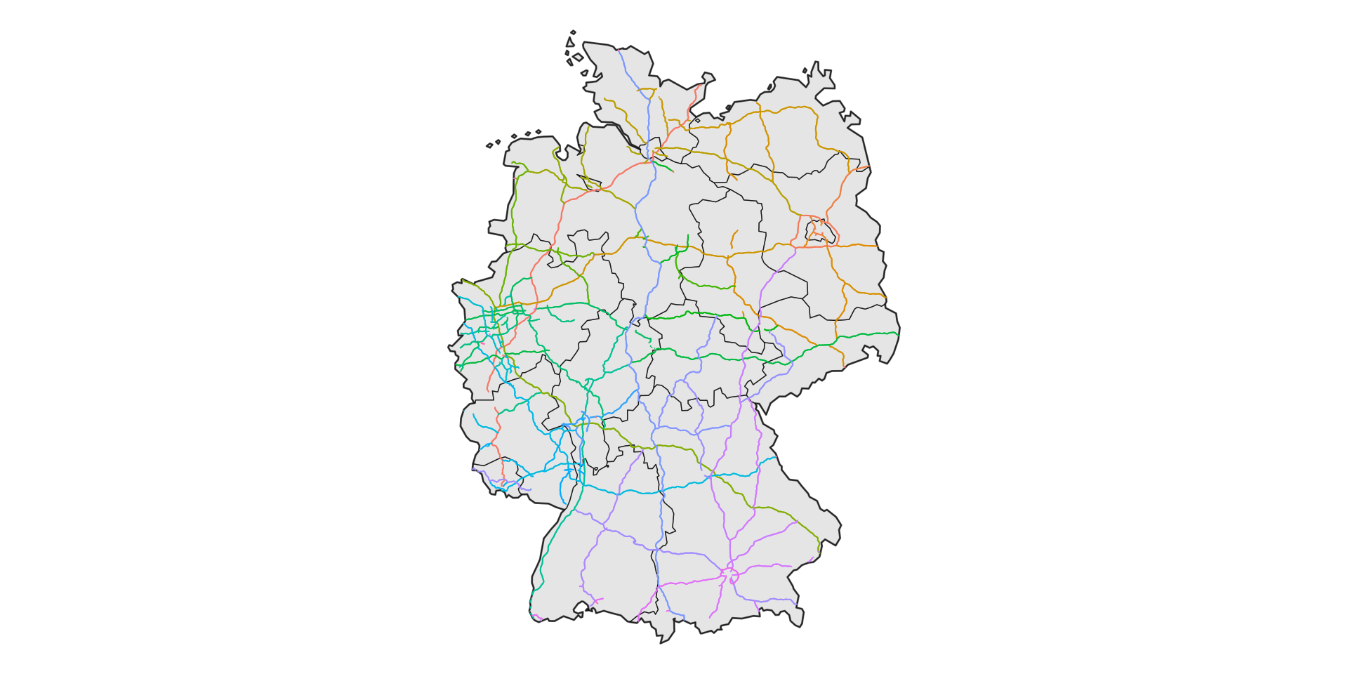

Zeichnen zusammen mit Karte

Ausschnitt festlegen: Möglichkeit 1/2

q <- opq(getbb("Bochum, Germany"))
s1 <-  add_osm_feature(q, key = "highway", value = "motorway") |> osmdata_sf()
ggplot() + geom_sf(data = s1$osm_lines) + coord_sf(xlim = c(7.17, 7.3), ylim = c(51.44, 51.5))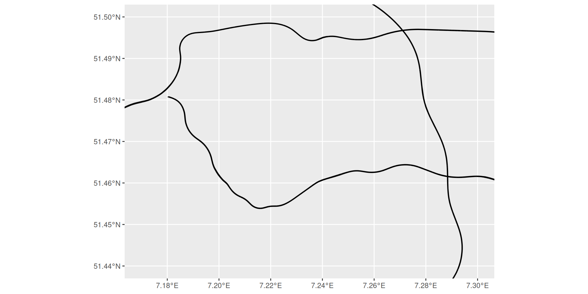

Ausschnitt mit coord_sf festlegen

Ausschnitt festlegen: Möglichkeit 2/2

q <- opq(c(7.17, 51.44, 7.3, 51.5))
s1 <- add_osm_feature(q, key = "highway", value = "motorway") |> osmdata_sf()
ggplot() + geom_sf(data = s1$osm_lines)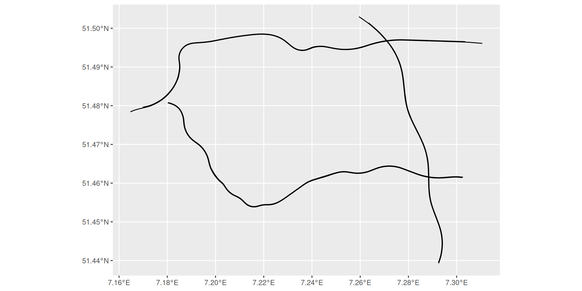

Ausschnitt der Anfrage bei opq angeben (und nicht mittels getbb)

Weitere hilfreiche Quellen zu OSM

8 Shapefiles

Shapefiles

d_wkr <- st_read("daten/Wkr_25833.shp", quiet = TRUE) |> st_transform(crs = "+proj=longlat")
ggplot(data = d_wkr) + geom_sf(mapping = aes(fill = Wkr), show.legend = FALSE)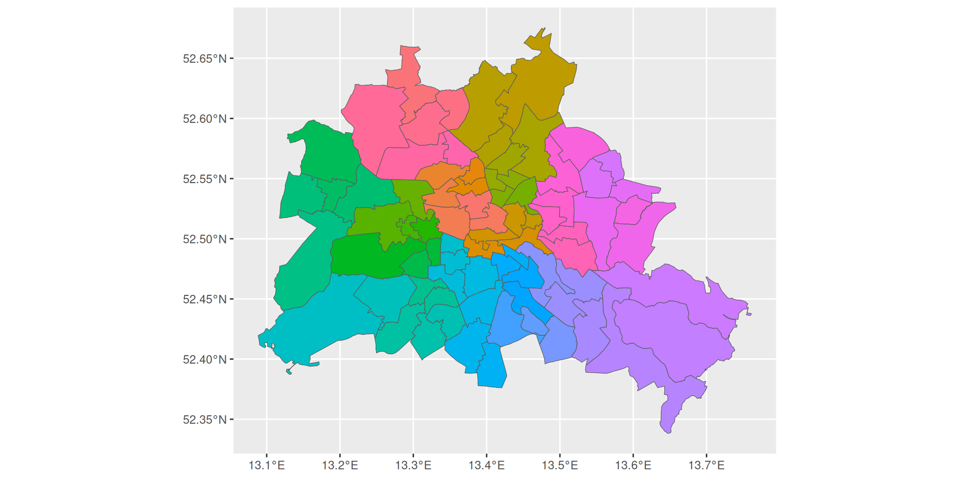

Dateiformat Shapefile (Endung .shp)
- Ursprünglich für ArcView (ESRI) entwickeltes Geodatenformat
Einlesen mit st_read()
Quelle

Räumliche Daten

1 Einführung

Räumliche Daten

Geographische Daten: Einzelne Punkte

Koordinatensystem mit Breiten- und Längengraden

GPS-Koordinaten Hochschule Bochum

Mercator-Projektion 1/2

Mercator-Projektion 2/2

Robinson-Projektion

Lambertsche Azimutalprojektion

Geographische Daten: Geometrien

Simple Features

R-Paket sf (Simple Features for R)

Paket sf: Simple Features in Dataframes

2 Weltkarte mit Natural Earth

Daten: Die Welt als Dataframe

Plot der Weltkarte

3 Berechnung neuer Daten

Weltkarte mit Fläche der Länder 1/2

Weltkarte mit Fläche der Länder 2/2

4 Kombination mit anderen Daten

Weltkarte mit der Lebenswerwartung

Dataframes miteinander verknüpfen

Weltkarte mit Lebenserwartung

5 Werte zu einzelnen Koordinaten

Erste Möglichkeit: Mit geom_point

Besser: Dataframe konvertieren und geom_sf

6 Landesgrenzen mit giscoR

Landesgrenzen Bundesrepublik 1/2

Landesgrenzen Bundesrepublik 2/2

7 Open Street Map

Über Open Street Map

Straßen in Bochum 1/2

Straßen in Bochum 2/2

Karte von Bochum 1/3

Karte von Bochum 2/3

Karte von Bochum 3/3

Bundesautobahnen 1/2

Bundesautobahnen 2/2

Ausschnitt festlegen: Möglichkeit 1/2

Ausschnitt festlegen: Möglichkeit 2/2

Weitere hilfreiche Quellen zu OSM

8 Shapefiles

Shapefiles

Erste Möglichkeit: Mit `geom_point`

Besser: Dataframe konvertieren und `geom_sf`

6 Landesgrenzen mit `giscoR`